

Analytical solution and numerical approaches of the generalized Leveque equation to predict the thermal boundary layer
ACI Avances en Ciencias e Ingenierías
Universidad San Francisco de Quito, Ecuador
Received: 25 October 2017
Accepted: 04 August 2018
Abstract: In this paper, the assumptions implicit in Leveque’s approximation are re-examined, and the variation of the temperature and the thickness of the boundary layer were illustrated using the developed solution. By defining a similarity variable, the governing equations are reduced to a dimensionless equation with an analytic solution in the entrance region. This report gives justification for the similarity variable via scaling analysis, details the process of converting to a similarity form, and presents a similarity solution. The analytical solutions are then checked against numerical solution programming by FORTRAN code obtained via using Runge-Kutta fourth order (RK4) method. Finally, others important thermal results obtained from this analysis, such as; approximate Nusselt number in the thermal entrance region was discussed in detail.
Keywords: Leveque approximation, Thermal entrance region, Thermal boundary layer, Dimensionless variables, Temperature, Nusselt number, Runge-Kutta method.
INTRODUCTION
The experimental studies carried out by the researchers are generally in the field of convective thermal transfers which several authors have addressed in their work, heat transfer problems in a flow of fully developed laminar fluid through circular conduits. An analysis of the heat transfers through a fluid flow and over the boundary layer was established by Hamad and Ferdows [1]. Another study was carried out by Wei and Al- Ashhab [2] on boundary layers of a non-Newtonian fluid subject to new boundary conditions. A study was conducted by Trimbijas et al. [3] to analyze a boundary layer in
mixed convection while employing a similarity technique to which partial differential equations are reduced to ordinary differential equations. Ahmed [4] analyzed a boundary layer in natural convection in the presence of transient wall temperatures using the finite difference method. Shen and Lu [5] have modeled the problem of free turbulence using the Runge-Kutta method for the prediction of the three-dimensional boundary layer. Mahanthesh et al. [6] carried out a heat flow analysis on the basis of a mathematical model managed by the boundary layer hypotheses while using the similarity method to reduce the governing equations. Eldesoky et al. [7] studied the peristaltic pumping of a compressible fluid in a tube using a perturbation analysis. Baehr and Stephan [8] and Stephan [9] conducted research on heat transfer in the input region with well-specified geometries. Additional work has been done by Asako et al. [10]. Shah and London [11], Kakac et al. [12], Ebadian and Dong [13], and Kakac and Yener [14] on triangular, rectangular and circular geometries. In the literature, we can find other thermal problems performed on other forms of tube geometries such as; the circular channels, the circular and the parallel plate and a rectangular channel. Thanks to these geometries, the thermal problems have been solved easily using analytical methods, of which whose prediction of the thermal transfer of the cylindrical walls was approached on several models. Hausen [15] developed a model to study the Graetz problem inside a circular tube. Churchill and Ozoe [16,17] proposed simple models to develop flux in a circular duct. With the fully developed asymptote, and for the thermal input region. The Leveque solution was combined by Churchill and Ozoe [16, 17]. For the Graetz problem, and in order to predict the thermal characteristics in an arbitrary form of the tube, models have been developed by Yilmaz and Cihan [18,19]. These two authors developed models for uniform wall flow conditions (H) and a uniform wall temperature (T) in order to predict the fully developed number of Nusselt. These models were fitted to these models with the Leveque generalized solution so that the input offers an approved model along the length of the tube. In the entrance area of the circular duct, two distinct problems must be considered. One assumes the existence of a fully developed hydrodynamic boundary layer while the other problem is more popular with developing thermal boundary layers. In the case of Graetz’s classical problem, the velocity distribution is fully developed and the temperature of the fluid tends to propagate fairly rapidly inside the tube. In the input region, the use of the Levèque approach gives us better convergent results in the approximate solution on which we can assume that the velocity gradient is quite linear and the boundary layer is considered thin. Belhocine and Wan Omar [20], Belhocine [21] conducted an analysis to predict the distribution of the dimensionless temperature in a fully developed laminar flow in a cylindrical pipe. Recently, Belhocine and Wan Omar [22] were able to develop the analytical solution of the problem of convective heat transfer within a pipe whose solution obtained is in the forms of the hypergeometric series.
The main objective of this work is to develop an exact solution of the thermal boundary layer at the inlet of a circular pipe for a fully developed flow of laminar fluid commonly called the Levèque approximation. The calculation methodology that we have followed is based on the method of solution in similarity of the variables in order to predict the dimensionless temperature as well as the thickness of the thermal boundary layer near the entrance of the flow. Several steps have been discussed here on the governing equation of the temperature field to reach the solution such that; the non- dimensionalization and the use similarity variables, the transform the PDE to a set of PDE’s. Summarization of the boundary conditions and the integration of the equation. We then compare the exact approximate solution of the levèque problem, with the numerical results using a Runge-Kutta fourth order (RK4) algorithm implemented by the FORTRAN code. The profiles of the solutions are provided from which we infer that the numerical and exact solutions agreed very well. Another result that we obtained from this study is the number of Nusselt in the thermal entrance region to which a parametric study was carried out and discussed well for the impact of the scientific contribution.
The governing heat diffusion equation
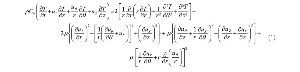
The total thermal energy balance, which is based on the use of equations of continuity and momentum, is simplified by the expression obtained by Bird, Stewart, and Lightfoot [23] is as follows;
The Graetz-Poiseuille flow problem
The Graetz problem consists of determining the temperature in a steady state of a fluid passing through a circular pipe whose flow is laminar fully developed. Thus, it is a transfer of heat by convection of a fluid approaching the inlet section of a cylindrical tube with a constant temperature T0 whose wall is subjected to a constant temperature Tw. The geometry of the problem is shown in Fig.1.
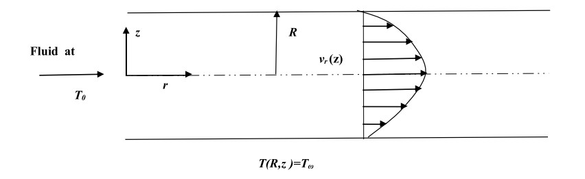
Illustration of Graetz problem
The contour of the velocity of the flow becomes a stable contour after a certain distance from the hydrodynamic inlet and it remains practically fully parabolic and invariable along the circular tube. Our context for solving the thermal problem is to find the behavior of the temperature field as it evolves to be uniform at the temperature of the downstream wall. The distribution of the velocity of the flow is not subordinated by the variation of the temperature as long as the nature of the fluid is incompressible.
The fluid flow is completely laminar in steady state and fully developed
The flow is considered incompressible Newtonian whose properties p, p, Cp, k. are constant and do not depend on temperature.
The temperature does not depend on the angular coordinate
Negligible viscous dissipation
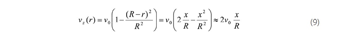
The expression of the velocity of a fully developed flow is given by the following form:
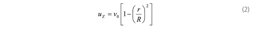
Where v0 is the maximum speed (center of the tube) , ur =0 , and uq =.0.
The energy equation is subject to the assumptions mentioned above, Eq.(1) can be written as follows:
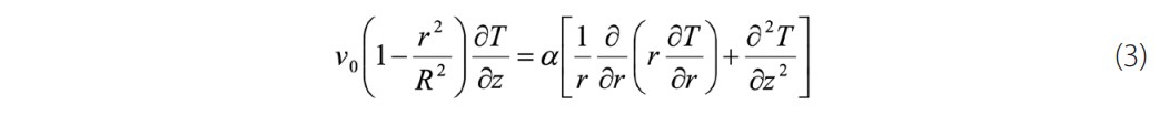
where is called the thermal diffusivity which has dimensions (m2/s), our problem is subjected to the following boundary conditions ; at the inlet of the tube ; at the wall of the tube and at the centerline is finite or .
Consider the following dimensionless terms:
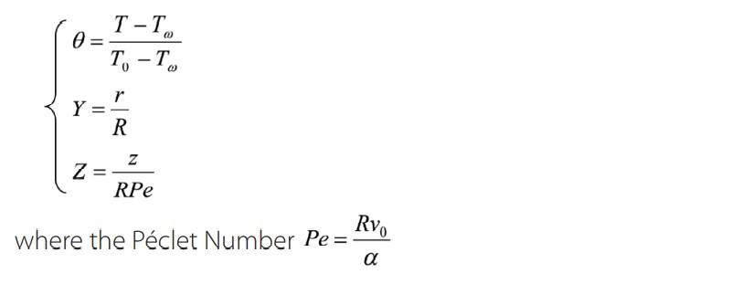
By substituting the variables T, r, z for their expressions as a function of the dimensionless variables θ, Y, Z in the heat equations, we obtain the following equations:
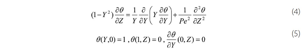
The influence of the axial diffusion is totally neglected when we apply the assumptions of the boundary layer, which implies the resolution of the following dimensionless equation

This equation can be solved by the technique of the separations of the variables at which the temperature that we seek will be found in terms of hypergeometric series
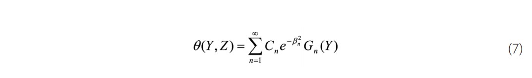
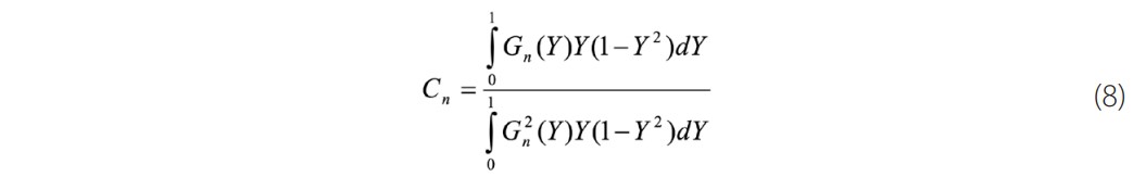
Where, and Gn(Y), are respectively the eigenvalues and the eigenfunctions associated with the Sturm-Liouville problems. The coefficients can be obtained by using the orthogonality property of the eigenfunctions defined as follows:
The Léveque Approximation
For all values of the axial position, the orthogonal function expansion solution obtained in the resolution of the classical Graetz problem is quite convergent, but the convergence is very slow as soon as one approaches the input tube. Indeed, for very long values of Z, the factor has become converged. Léveque [24] examined the thermal input zone in a cylindrical pipe while developing an approximate solution which is formally advantageous when the orthogonal function tends towards convergence to gradually (Fig.2).
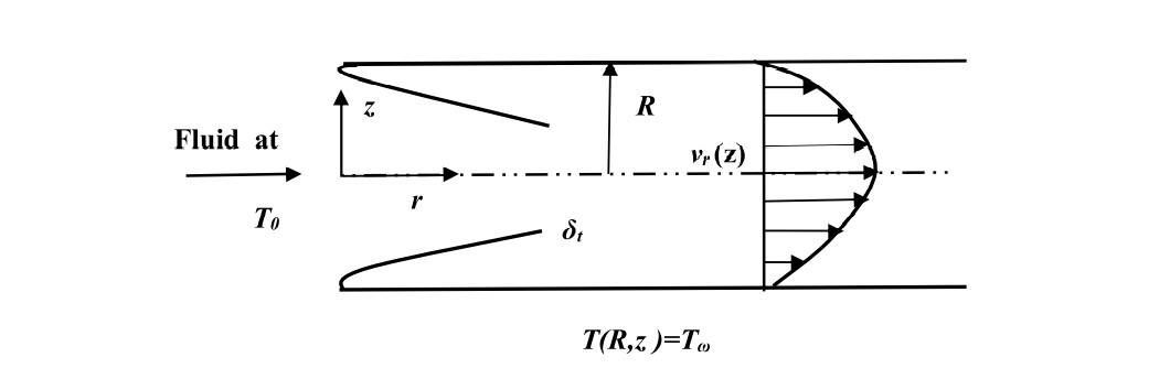
Simplifying representation of the Lévêque approximation
According to Leveque’s assumption, we can take the thickness of the boundary layer , which leads to the following simplifications:
In the radial conduction term, we can neglect here the effects of curvature. Thus, derivative is approximated by
We are interested in the thermal boundary layer of the velocity allocation of which it can be developed in a Taylor series from the wall of the pipe according to a measured position, if we keep the first non-zero term.
If we set x=R-r, the speed distribution will take the following form:
Let us know, the boundary conditions of the flow entering the pipe are those that lie outside the boundary layer, we will exploit the boundary condition T(x→∞)→t0 instead of that market at the center of the tube to arrive at the Graetz solution.
Governing Lévéque’s Equation
Starting from the reduced energy equation whose axial conduction has been neglected yet, and considering the said hypotheses, for the temperature field, we obtain the following governing equation

Using the string rule, in order to convert the second derivative of r into that of x, we get

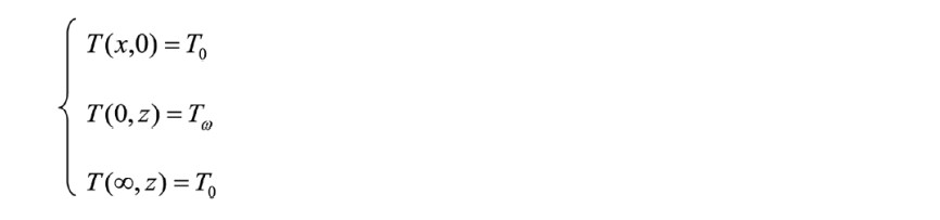
Boundary Conditions
The temperature T(x, z), is controlled by boundary conditions which are fixed like this.
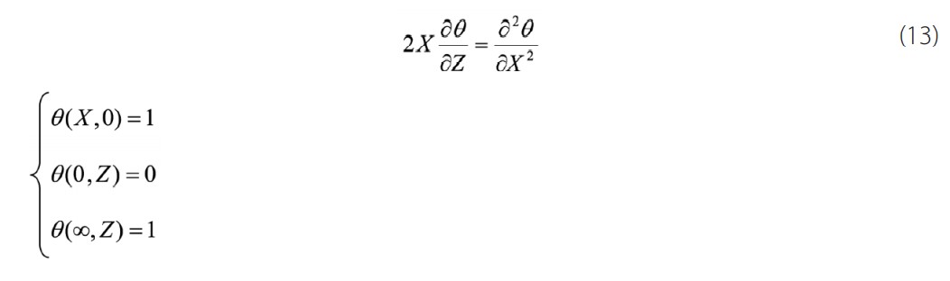
Non-Dimensionalization
Now, we will use dimensionless variables for the simplification of the equation. For this, we introduce the temperature and the axial coordinate of the following forms

The scaled governing equation placed on the wall by X=x/R and boundary conditions are given as follows
Analytical Methodology for Problem Solving: Temperature Field and Thermal Boundary Layer
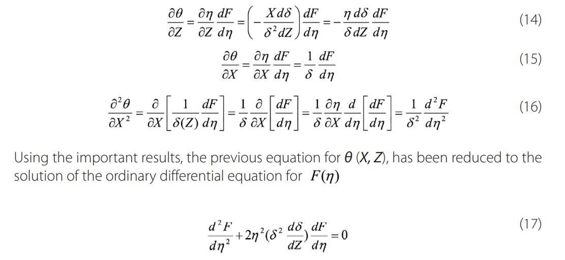
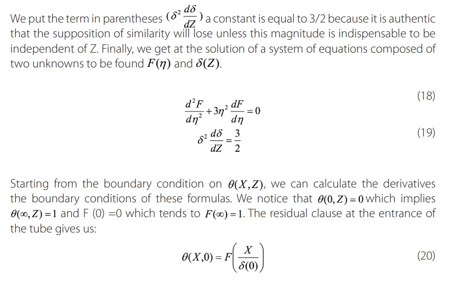
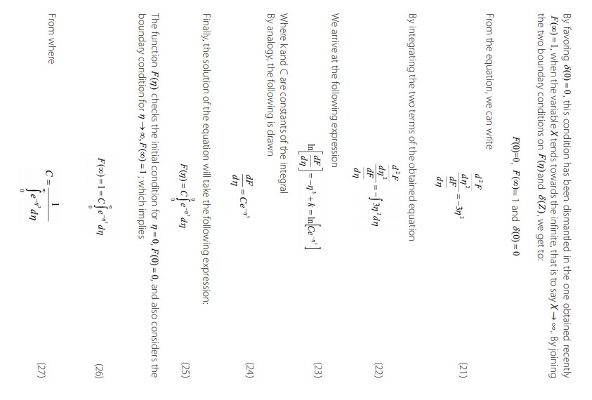
|f a similarity solution exists for a given situation, a mathematical transformation of coordinate systems can be performed to reflect this fact. A similarity technique converts these partial differential equations to ordinary differential equations and therefore, make the solution much more simple. These analytical solutions still require numerical integrations. At the current problem, we are looking for a similarity solution for the temperature field, we assume, , where is the similarity variable and is variable represents the scaled thermal boundary layer thickness, and is unknown at this stage. Using the chain rule, we will perform the following necessary transformations.
Numerical resolution of the problem using RK04 method
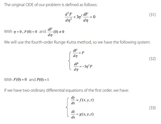
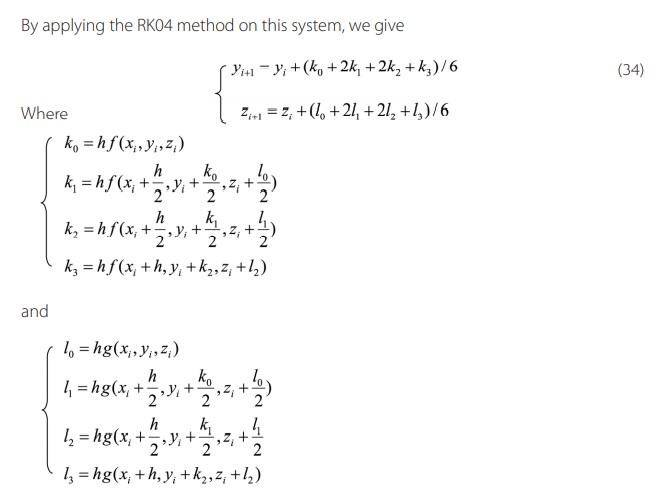
We have adopted the Kutta Runge algorithm for finding the solution of our system of equations;
The interval for the integration of the equations is chosen to perform our calculations: [a, b] if we take a = 0, and b = 3
The number of iterations N = 30,
The size of the iterations will be estimated as follows: h = (b-a) /N=3/30=0.1
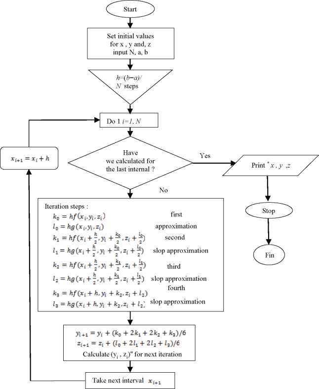
Flowchart of the RK-4 method for resolving the second ODE’s systems.
The main program was drafted by FORTRAN, which will solve the problem of Leveque whose procedure initiated to solve simultaneously two differential equations of the order by the method of Runge Kutta RK04. This program relies on a definition of two functions whose subroutine RK04 is called at each repetition of the loop that intervenes in the calculations. The code edited in the machine that was executed is illustrated in detail in Figure 4.
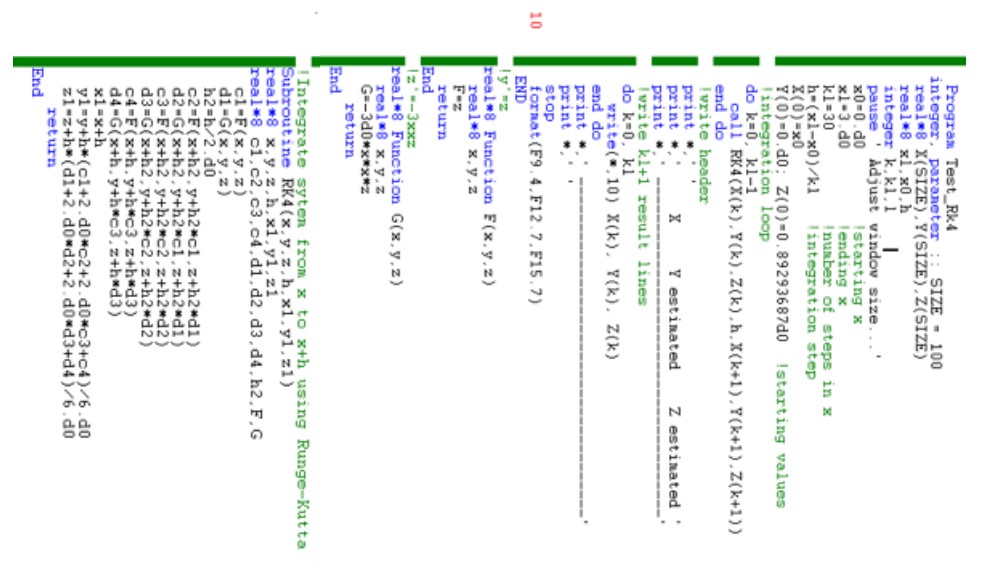
FORTRAN code of Runge Kutta for set of first order differential equations
RESULTS AND DISCUSSIONS
Validation of the numerical results via the analytical solution of the problem
The analytical solution that we have developed above is compared here with the numerical results derived from the FORTRAN V.05 calculation code. The results of the two methods are condensed in detail in Table 1.
| Variable n | Exact analytical solution F( n ) | Runge-Kutta (RK4) method F( n ) |
| 0 | 0 | 0.0000000 |
| 0,1 | 0,08927136 | 0.0892714 |
| 0,2 | 0,17823109 | 0.1782309 |
| 0,3 | 0,26608715 | 0.2660866 |
| 0,4 | 0,35156264 | 0.3515626 |
| 0,5 | 0,43300027 | 0.4329998 |
| 0,6 | 0,50853023 | 0.5085291 |
| 0,7 | 0,57631574 | 0.5763146 |
| 0,8 | 0,63483615 | 0.6348343 |
| 0,9 | 0,68314582 | 0.6831438 |
| 1 | 0,72105634 | 0.7210538 |
| 1,1 | 0,74916957 | 0.7491656 |
| 1,2 | 0,76875346 | 0.7687482 |
| 1,3 | 0,78149478 | 0.7814872 |
| 1,4 | 0,78918921 | 0.7891808 |
| 1,5 | 0,79347888 | 0.7934697 |
| 1,6 | 0,79567283 | 0.7956641 |
| 1,7 | 0,79669613 | 0.7966892 |
| 1,8 | 0,79712921 | 0.7971242 |
| 1,9 | 0,7972944 | 0.7972914 |
| 2 | 0,79735155 | 0.7973494 |
| 2,1 | 0,79736852 | 0.7973676 |
| 2,2 | 0,79737298 | 0.7973729 |
| 2,3 | 0,79737387 | 0.7973742 |
| 2,4 | 0,79737387 | 0.7973746 |
| 2,5 | 0,79737477 | 0.7973747 |
| 2,6 | 0,79737477 | 0.7973747 |
| 2,7 | 0,79737477 | 0.7973747 |
| 2,8 | 0,79737477 | 0.7973747 |
| 2,9 | 0,79737477 | 0.7973747 |
| 3 | 0,7973747 | 0.7973747 |
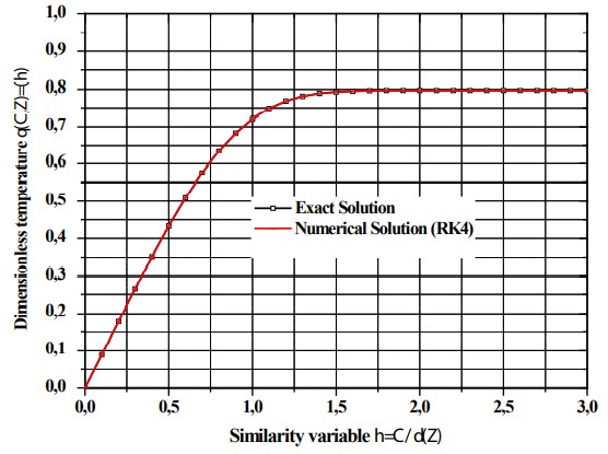
Exact results and the numerical solution
Fig. 5 shows a comparison between the resolution results of the equation predicted by the analytical method and the numerical data derived from the FORTRAN code, the two sets of results of which are plotted in the same figure. On the basis of Fig. 5, it can be seen that the two curves are fairly identical, while observing that the dimensionless temperature θ gradually and gradually increases to the abscissa Z = 0.7, then loops and arches a little, by varying its path until it reaches the position Z = 1.7 where it stabilizes at a constant value 0.79 along the tube until the outlet of the fluid stream. Fig. 5 shows clearly that the results of the analysis solution are very excellent convergence with those of the numerical results performed by the Visual FORTRAN v5.0 calculation code during which the use of the RK04 method obviously gives us a severely accurate assessment.
Comparison of exact and fourth-order Runge Kutta (RK4) numerical solutions
Fig.6. shows the variation in the thickness of the thermal boundary layer as a function of the longitudinal coordinate where the latter increases slowly from the zero position towards the direction of flow of the fluid as it penetrates the pipe through its center and arrogates its total space. At the inlet of the tube and its wall, the shear stress is greater during which the thickness of the boundary layer is very short and slowly decreases to the fully developed value. In fact, the collapse of the pressure is increased in the inlet zone of the tube under the effect which may cause the phenomenon of friction over the whole of the tube. This elevation can be negligible for long and important tubes in short lengths. A thin layer can be observed on the wall at which the velocity of flow is less than the wall. By going from front to back, the thickness of the thermal boundary layer lengthens along the channel.
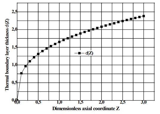
Thermal boundary layer thickness distribution by analytical method
The heat transfer coefficient
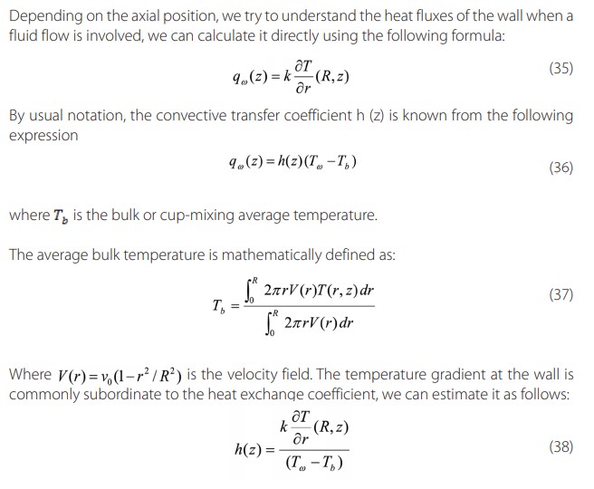
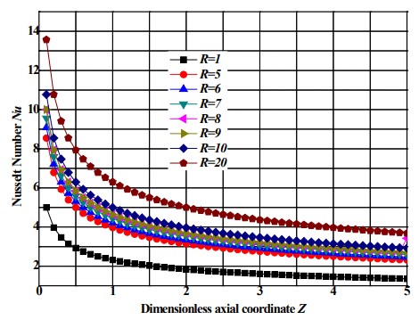
Fig.7 shows the variation obtained in the input region of the Nusselt number as a function of the axial distance Z obtained in the thermal input region for various radius of the pipe. We can observe that the number of Nusselt, Nu (Z), rises as a function of the increase of the radius of the tube and that this influence is very noticeable enlarged at the entrance. When Z is greater than a certain distance, all the bundles of curves have become intensified and they stabilize horizontally flat, this explains why the fully developed boundary layer is reached. Indeed, the boundary layer triggers to increase when the fluid enters the tube in the walls of the walls having a temperature distinct from that of the fluid. The developed thermal condition is achieved after the flow passes a certain position.
Nusselt number as a function of axial position for different tube radius
Fig. 8 shows the Nusselt number as a function of the longitudinal coordinate for different values of the Peclet number. It is observed that the increase in the number of Peclet leads to an increase in the number of Nusselt. As can be seen, the Péclet number has a much more pronounced effect on the Nusselt values for positions near the tube entrance. However the curve exhibits the same overall behavior - larger Nu at small Z and more or less constant value of large Z. In the tube entry region, where the boundary layer has expanded, we can see the reduction of the Nusselt number where it stabilizes in the fully developed thermal zone to a constant value does not depend on the Reynolds number and the heat flux. Hence, the thermal coefficient (h) appeared unlimited at the birth of the thermal boundary layer, and then gradually decreases to a stable value when the flow is fully developed at the origin. The numerical results clearly illustrate that the value ofthe Nusselt number increases and then decreases sharply over the entire longitudinal position of the tube.
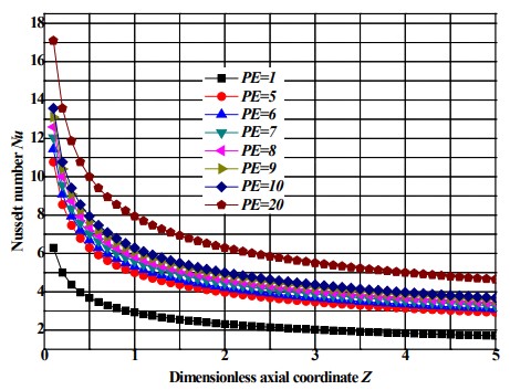
Nusselt number as a function of axial position with various Peclet numbers
In conclusion, this paper presented an analytical and numerical solution to the Leveque approximation problem in order to predict the evolution of the thickness of the boundary layer as well as the temperature of the fluid at thermal entrance fully developed region through a circular tube with boundary condition at the axial coordinate origin. The exact solution methodology was based on the similarity variable and the generalized integral transform technique while the numerical approach is based on the integration technique of two differential equations with the Runge Kutta method of order 4 (RK4) programmed in Visual FORTRAN v5.0. The solution method was verified to lead to converging values which are in accordance with physically expected results. After demonstrating the convergence of the solution, the Nusselt number distribution of different Peclet values was analyzed, and the results are also in accordance with expected literature values. As final comments one should mention that the same solution procedure can be used for any dynamically developed velocity profile, as it occurs in many other occasions. Also, the methodology can be easily extended to other configurations such as another channel geometries, different wall heating conditions, and vicious and other flow heating effects.
References
[1] Hamad ,M. A. A., Ferdows , M.(2012).Similarity solutions to viscous flow and heat transfer of nanofluid over nonlinearly stretching sheet, Applied Mathematics and Mechanics (English Edition) ,33(7), 923-930. doi 10.1007/s10483-012-1595-7.
[2] Wei, D. M., Al-ashhab, S.(2014). Similarity solutions for non-Newtonian power-law fluid flow, Applied Mathematics and Mechanics (English Edition),35(9), 1155-1166 , doi 10.1007/s10483-014-1854-6
[3] Trimbijas, R., Grosan, T., Pop, I. (2015). Mixed convection boundary layer flow past vertical flat plate in nanofluid: case of prescribed wall heat flux, Applied Mathematics and Mechanics (English Edition),36(8), 1091-1104 , doi 10.1007/ s10483-015-1967-7
[4] Ahmed ,S. E.(2017). Modeling natural convection boundary layer flow of micropolar nanofluid over vertical permeable cone with variable wall temperature, Applied Mathematics and Mechanics (English Edition),38(8) ,1171-1180, doi 10.1007/s10483-017-2231-9
[5] Shen,L., and Lu,C.(2017). Mechanism of three-dimensional boundary-layer receptivity, Applied Mathematics and Mechanics (English Edition), 38(9) ,1213-1224, doi 10.1007/s10483-017-2232-7
[6] Mahanthesh ,B., Gireesha ,B. J., Shehzad ,S. A., Abbasi ,F. M. , Gorla ,R. S. R. (2017).Nonlinear three-dimensional stretched flow of an Oldroyd-B fluid with convective condition, thermal radiation, and mixed convection. Applied Mathematics and Mechanics (English Edition), 38(7), 969-980, doi 10.1007/s10483-017-2219-6
[7] Eldesoky ,I. M., Abdelsalam ,S. I., Abumandour ,R. M., Kamel ,M. H. , Vafai ,K.(2017). Interaction between compressibility and particulate suspension on peristaltically driven flow in planar channel. Applied Mathematics and Mechanics (English Edition), 38(1), 137-154, doi 10.1007/s10483-017-2156-6
[8] Baehr, H., Stephan, K.(1998). Heat Transfer, Springer-Verlag.
[9] Stephan, K., (1959) Warmeubergang und Druckabfall bei Nicht Ausgebildeter Laminar Stromung in Rohren und in Ebenen Spalten,’ Chemie-Ingenieur-Technik, 31(12), 773-778
[10] Asako, Y., Nakamura, H., Faghri, M , (1988). Developing Laminar Flow and Heat Transfer in the Entrance Region of Regular Polygonal Ducts, International Journal of Heat Mass Transfer,31(12), 2590-2593
[11] Shah, R. K., London, A. L. (1978). Laminar Flow Forced Convection in Ducts, Academic Press, New York, NY,
[12] Kakac, S., Shah, R. K., Aung, W. (1987). Handbook ofSingle Phase Convective Heat Transfer, Wiley, New York,
[13] Ebadian, M.A. Dong, Z.F. (1998). Forced convection internal flows in ducts, In: Handbook of heat transfer,3rd Edition, McGraw-Hill, New York, 5.1-5.137
[14] Kakac, S., Yener, Y. (1983) ‘‘Laminar Forced Convection in the Combined Entrance Region of Ducts,’’ in Low Reynolds Number Heat Exchangers, S. Kakac, R. K. Shah and A. E. Bergles, eds., Hemisphere Publishing, Washington, 165-204
[15] Hausen, H.(1943).“Darstellung des Wärmeübergangs in Rohren durch verallgemeinerte Potenzbezie-hungen”, VDI- Zeitung, Suppl. “Verfahrenstechnik”, 4, 91-98
[16] Churchill, S. W., Ozoe, H. (1973). ‘‘Correlations for Laminar Forced Con-vection with Uniform Heating in Flow Over a Plate and in Developing and Fully Developed Flow in a Tube,’’ ASME J. Heat Transfer,95, 78 - 84
[17] Churchill, S. W., Ozoe, H., (1973). ‘‘Correlations for Laminar Forced Con-vection in Flow Over an Isothermal Flat Plate and in Developing and Fully Developed Flow in an Isothermal Tube,’’ ASME J. Heat Transfer,95, 416 - 419
[18] Yilmaz,Cihan.E. (1993). ‘’General equation for heat transfer for laminar flow in ducts of arbitrary cross-sections’’, International Journal of Heat and Mass Transfer, 36(13), 1993, 3265-3270
[19] Yilmaz.T, Cihan.E. (1995). ‘‘An Equation for Laminar Flow Heat Transfer for Constant Heat Flux Boundary Condition in Ducts of Arbitrary Cross-Sectional Area’’,J. Heat Transfer 117(3), 765-766
[20] Belhocine, A. , Wan Omar, W. Z.(2016). ‘’Numerical study of heat convective mass transfer in a fully developed laminar flow with constant wall temperature’’, Case Studies in Thermal Engineering, 6, 116-127
[21] Belhocine, A. (2016). ‘’Numerical study of heat transfer in fully developed laminar flow inside a circular tube’’. International Journal of Advanced Manufacturing Technology. 85(9):2681-2692, doi 10.1007/s00170-015-8104-0
[22] Belhocine.A, Wan Omar, W.Z. (2017). An analytical method for solving exact solutions of the convective heat transfer in fully developed laminar flow through a circular tube, Heat Transfer—Asian Research, 46(8), 1342-1353 ,doi: 10.1002/htj.21277
[23] Bird, R.B., Stewart, W.E., Lightfoot, E.N. (1960). ‘’Transport Phenomena’’, John Wiley and Sons, New York,
[24] Lévêque, M.A. (1969). ‘’Les lois de la transmission de chaleur par convection’’, Annales des Mines, Memoires, Series 12, 13, 201-299, 305-362, 381-415 (1928) {as cited by J. Newman, Trans. ASME J. Heat Transfer, 91, 177.
[25] Abramowitz, M., Stegun, I. (1965). Handbook of Mathematical Functions, Dover, New York.
Additional information
AUTHOR’S CONTRIBUTIONS: Ali Belhocine
conceived the research, conducted the survey, analyzed the data, interpreted
the results and wrote the document while Wan Zaidi Wan Omar, as my co-author,
contributed in the present research, revised the manuscript critically and
collaborated with editing.