

Pruebas
Spectral discretizations of the Darcy’s equations with non standard boundary conditions
ACI Avances en Ciencias e Ingenierías
Universidad San Francisco de Quito, Ecuador
Received: 27 February 2017
Accepted: 09 July 2021
Abstract: This paper is devoted to the approximation of a nonstandard Darcy problem, which modelizes the ow in porous media, by spectral methods: the pressure is assigned on a part of the boundary. We propose two variational formulations, as well as three spectral discretizations. The second discretization improves the approximation of the divergence-free condition, but the error estimate on the pressure is not optimal, while the third one leads to optimal error estimate with a divergence-free discrete solution, which is important for some applications. Next, their numerical analysis is performed in detail and we present some numerical experiments which conrm the interest of the third discretization.
Keywords: Spectral methods, Darcy equations, boundary conditions, numerical results.
Introduction
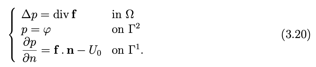
We consider the following Darcy problem:
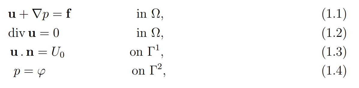
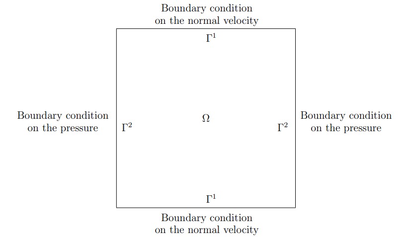
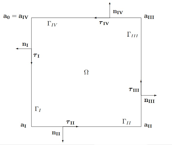
where Ω is the plane square ] — 1, 1[2 and n = (n 1 ,n2) is the exterior unit normal to the boundary Γ = ∂Ω. The boundary Γ is divided into two parts: the horizontal portion Γ1 = {(x,y)| — 1 < x < 1 ,y = ± 1} and the vertical portion Γ2 = {(x,y)|x = ± 1, — 1 < y < 1}. As we can see, the boundary condition on Γ2 are nonstandard, since we prescribe the value of the pressure on Γ2. On the contrary, we have a classical condition on the portion Γ1. These conditions are described in the following figure.
Boundary condition on the normal velocity
The equations of the Darcy problem not only modelize the flow in porous media, but also appear in the projection techniques for the solution of Navier-Stokes equations (see [10] and [15]). The nonstandard boundary conditions, where the pressure is assigned on a part of the boundary, have a physical meaning: typically the portion Γ1 corresponds to rigid walls, whereas the entry or exit of the fluids takes place through Γ2. The spectral discretization with this type of boundary conditions was only studied within the framework of the Stokes problem (see [6], [4] and [5]), while Azaiez, Bernardi and Grundmann proposed in [2] the spectral discretization of the standard Darcy problem, where the normal velocity is assigned on the boundary.
This paper is devoted to the spectral discretization of the nonstandard Darcy problem. First, we give two variational formulations. Each one leads us to well-posed problems. Second, we study the regularity of the solution by using a mixed problem of Dirichlet- Neumann for the Laplace operator. Next, from the first variational formulation, we derive a first spectral discretization, which is simple, but, in order to improve the approximation of the divergence-free condition, we study a second spectral discretization, where the inf-sup condition is obtained with more difficulty and where the error estimate on the pressure is not optimal. Finally, the second variational formulation yields a third spectral discretization, which leads us to optimal error estimate and a divergence-free discrete solution.
An outline of this paper is as follows. The two continuous variational problems, as well as the regularity of the solution, are studied in Section 2. Section 3 is devoted to the analysis of three spectral approximations of this problem in the case of homogeneous boundary conditions. In Section 4, we present the algorithms that are used to solve the first and third discretizations, together with some numerical experiments.
Statement of the problem and notation
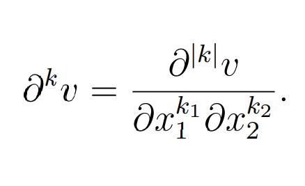
In order to set this problem into adequate spaces, recall the definition of the following standard Sobolev spaces (cf. J. Necas [13]). For any multi-index k = (k1 ,k2) with ki > 0, set |k| = k1 + k2 and denote
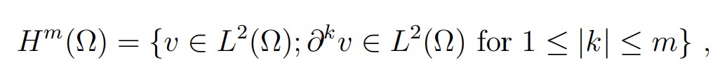
Then for any integer m ≥ 0 and any plane domain Ω whose boundary is Lipschitz continuous(cf. Grisvard [12]), we define:
equipped with the seminorm
and norm(for which it is an Hilbert space)
For extensions of this definition to non-integral values of m (see [11,12]), let s a real number such that s = m + σ with m ∈ N and 0 <σ< 1. We denote by Hs(Ω) the space of all distributions u defined in Ω such that u ∈ Hm(Ω) and, ∀|α| = m,
It can be shown that Hs(Ω) is a Hilbert space for the scalar product

Let Γ' be an open part of the boundary ∂Ω of class Cm−1,1 and the mapping defined on Hm(Ω). We denote by (see [7,12]) the space (Hm(Ω)) which is equipped with the norm:

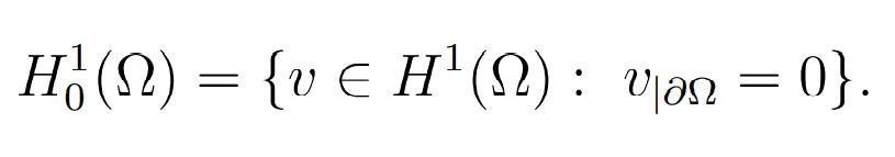
In this text, we shall use the spaces H1/2(Γ') and H3/2(Γ') corresponding to m = 1 and 2. Let us define the space H1/200 (Γ') = {v|Γ', v ∈ H1(Ω), ∀x ∈ ∂Ω \ Γ ', v|∂Ω(x)=0}. We shall also be interested in the dual space of H1/200 (Γ'),

We shall use the Hilbert space H(div ; Ω) = {v ∈ L2(Ω)2 : div v ∈ L2(Ω)}, equipped with the norm
For vanishing boundary values, we define:
For Λ =]−1,1[ , we denote the norm in L2(Λ) by , the seminorm in H1(Λ)and the norm in H1(Ω) by .
We note x = (x,y) the generic point of the square Ω and we call ΓI, ΓII , ΓIII and ΓIVthe edges of Ω, starting from west and turning counterclockwise. For each J, J = I,II,III,IV, the extremities of the edge ΓJ are aJ-1 and aJ, with the convention ao = aIV, the exterior unit normal vector to ΓJis denoted by nJ and the counterclockwise unit tangent vector is . Figure 1.2 below presents this notation.
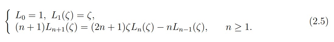
For any domain Δ in R or R2 and for any nonnegative integer n, Pn(Δ) stands for the space of all polynomials on Δ with degree < n with respect to each variable. We also use the notation P0n(Δ) for the subspace Pn(Δ) ∩ H10(A). For ∆ =]-1, 1[, the family (Ln)n of Legendre polynomials is a basis of the spaces P() of polynomials on (we refer to [7, Chap. I] for the properties of the orthogonaI poIynomiaIs). These poIynomiaIs are orthogonal to each other in L2( ) and are caracterized as follows: for any integer n > 0, the polynomial Ln is of degree n and satisfies Ln(1) = 1. Let us recall some properties that we need. The family (Ln)n is given by the recursion relation:
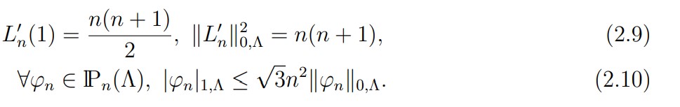
Each polynomial is a solution of the differential equation

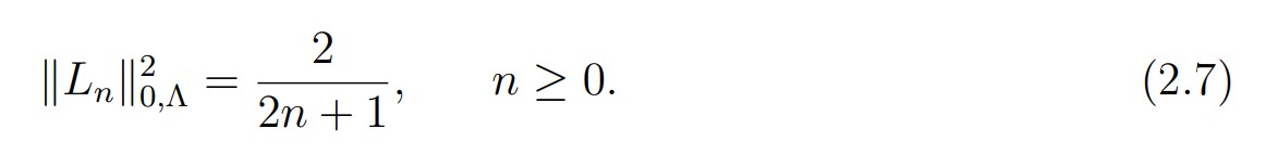
and its norm is given by
Three consecutive polynomials are linked by the integral equation
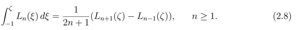
From (2.6) and integration by parts, we derive
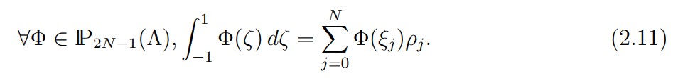
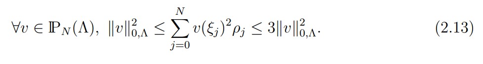
Next, let N ≥ 2 be a fixed integer. We denote by ξj , 0 ≤ j ≤ N, the zeros of the polynomial (1 − ζ2)L N (ζ) in increasing order. We recall (see [7, Chap. I]) that there exist positive weights ρj , 0 ≤ j ≤ N, such that the following equality, called the Gauss-Lobatto formula, holds
Moreover, it follows from the identity (see [7, Chap. III])
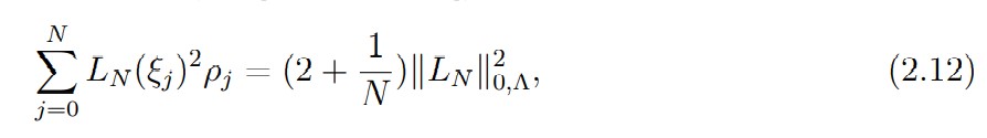
that the bilinear form: is a scalar product on PN (Λ), since we have
THE CONTINUOUS PROBLEM
First variational formulation
We define the subspace H 1(Ω; Γ') = {v ∈ H 1(Ω)|v = 0 on Γ'} of H 1(Ω) and we introduce the space:

In the same way as in [1], we consider the following equivalent variational formulation of the problem (1.1)-(1.4):
Find u in L2(Ω)2and p in H1(Ω) such that p − ϕ belongs to M and that
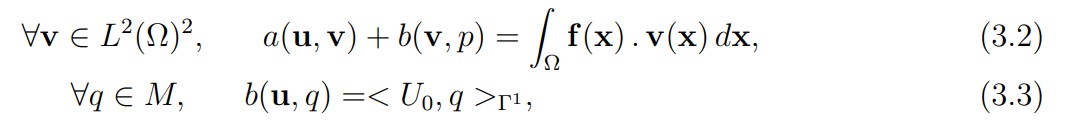
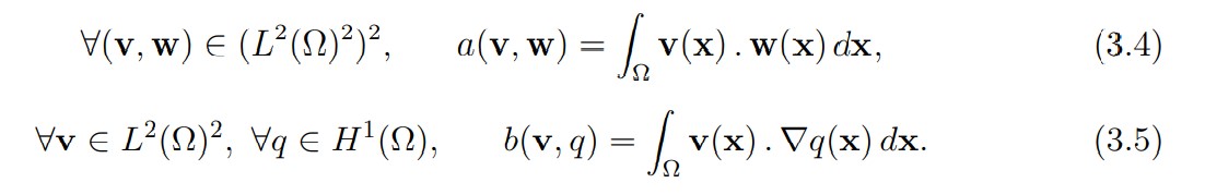
where the bilinear forms a and b are defined by
Theorem 3.1Let fbe in L2(Ω)2, U0 in H−1/2(Γ1) and ϕ in H1/2(Γ2), where H−1/2(Γ1) and H1/2(Γ2) are defined respectively in (2.3) and (2.2). Then problem (3.2), (3.3) has a unique solution satisfying

Proof. First, let us define φ ̃ belonging to H1/2(Γ) such that φ ̃|Γ2 = φ and || φ ̃||1/2,Γ ≤ c|| φ ||1/2,Γ2 . To this end, we must extend ϕ to a function belonging to H1/2(Γ). Let µ be a function defined in [0, 2] by
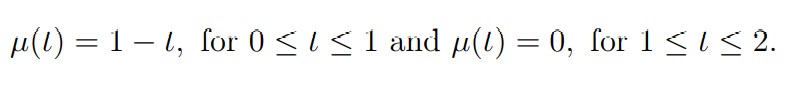
We define φ ̃|Γ11 by

and φ ̃|ΓIV by

Then we have ∥φ ̃∥1/2,Γ ≤ C∥φ∥1/2,Γ2 . Next, let Φ in H1(Ω) such that Φ|Γ = φ ̃. Finally, we obtain a function Φ verifying

Second, let us extend U0 to a function belonging to H−1/2(Γ). We set U ̃0|Γ1 = U0 and U ̃0|Γ2 = −1/2 < U0,1 >Γ1 . Then, we have ∥U ̃0∥−1/2,Γ ≤ C∥U0∥−1/2,Γ1 and < U ̃0,1 >Γ= 0. Next, we define Neumann’s Problem:
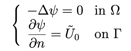
and we set u0 = ∇ψ. Applying Proposition 1.2 of [11, page 14], we derive that ψ belongs to H1 (Ω), which implies that u0 belongs to H (div ; Ω) with
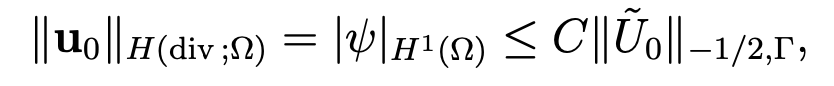
since div uo = ∆ψ = 0. Finally, u0 verifies

Now, let us split p as: p = Φ + p ̃ with p ̃ in M and u as: u = u0 + u ̃. Then, we can write the problem (3.2),(3.3) as


Since the right-hand side of (3.9) defines a continuous form on L2(Ω)2 and since the properties of continuity and ellipticity are obvious we have only to check the following inf-sup condition on the form b (see [11, pages 58,59]):

with a positive constant β. This ”inf-sup condition” was introduced independently by Babuska [3] and Brezzi [9]. We can verify this condition by taking v = ∇q . Indeed, we have
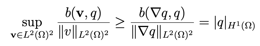
and, since q|Γ2 = 0, using a generalization of Poincar ́e inequality (see [11, Chap. I, page 40]) yields ∥q∥L2(Ω) ≤ P|q|H1(Ω), which implies
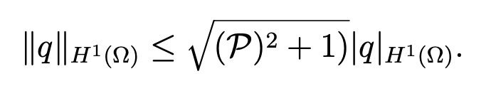
Thus, the ”inf-sup condition” is verified with the positive constant β = 1/√ (P)2 + 1). Hence, applying Theorem 2.3 [7, pages 116,117], the theorem follows.
Second variational formulation
We introduce the space:

In an analogous way as in [1], we consider the following equivalent variational formulation of the problem (1.1)-(1.4):
Find u in X and p in L2(Ω) such that u − u0 belongs to X, where u0 is the function previously constructed that verifies (3.8), and that


where the bilinear form b∗ is defined by

In the same way as previously, we split u as: u = u0 + u ̃. Then, we can write the problem (3.13),(3.14) as


Since the right-hand side of (3.16) defines a continuous form on X and since the properties of continuity and ellipticity are obvious, we have only to check the following inf-sup condition on the form b∗:
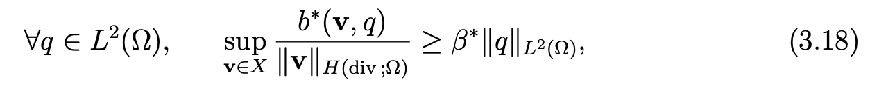
with a positive constant β∗. Let us note that  belongs to L20(Ω) and, owing to a classic result (see [11, Chap. I]), there exists v0 in H10(Ω)2, such that

Then, we set

We can verify that v ̃ belongs to X with

since  Then, we have
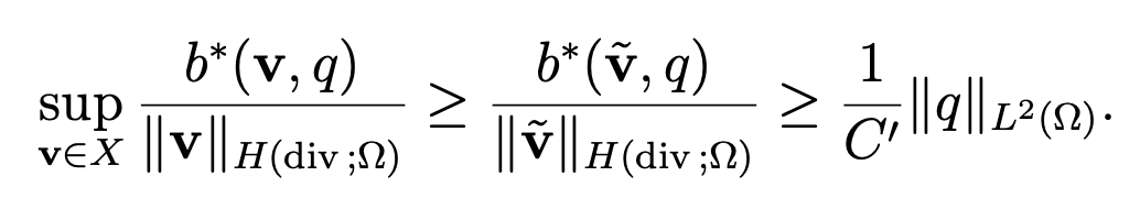
Hence, we derive the inf-sup condition and we obtain the following result.
Theorem 3.2Let fbe in L2(Ω)2, U0 in H−1/2(Γ1) and φ in H1/2(Γ2), where H−1/2(Γ1) and H1/2(Γ2) are defined respectively in (2.3) and (2.2). Then problem (3.13), (3.14) has a unique solution satisfying

Regularity results
When the data f is in H (div ; Ω), taking the divergence of the first equation of the problem (1.1)-(1.4) and owing to the other equations, we obtain a mixed problem of Dirichlet-Neumann for the Laplace operator:
We suppose that f is in H1(Ω)2, φ is in H3/2(Γ2) and U0 is in H1/2(Γ1). In addition, we assume matching conditions at the vertices of Γ (see [7, Chap I]):
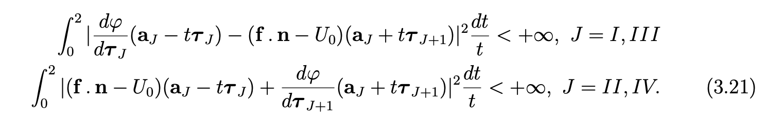
Theorem 3.3For any data f in H1(Ω)2, φ in H3/2(Γ2) and U0 in H1/2(Γ1), where H3/2(Γ2) and H1/2(Γ1) are defined in (2.2) , verifying the matching conditions (3.21), the solution (u, p) of the problem (1.1)-(1.4) belongs to H1(Ω)2 × H2(Ω).
Proof. Owing to matching conditions (3.21), there exists p0 in H2(Ω) such that p0|Γ2 = φ and (∂p0/∂n)|Γ1 =f.n−U0. Let us set p ̃=p−p0. The problem (3.20) is equivalent to the following problem: find p ̃ in H1(Ω; Γ2) such that

Since the boundary between Γ1 and Γ2 is the set of vertices of Γ, the regularity of the data implies that this homogeneous mixed problem of Dirichlet-Neumann for the Laplace operator has a solution p ̃ in H2(Ω) (see [12]). Hence, we derive the regularity of p and u. ♦
Remark 3.4If (f . n−U0) is Lipschitz-continuous on ΓJ or belongs to H1(ΓJ ), J = II, IV and if φ belongs to C1,1 (ΓJ) or to H2 (ΓJ), J = I, III, the matching conditions (3.21) are equivalent to simpler conditions:

SPECTRAL DISCRETIZATION
First spectral discretization
We define the discrete scalar product by
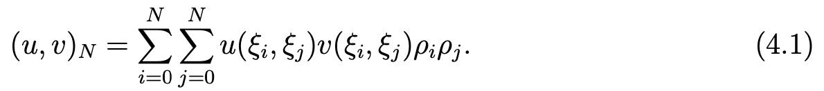
and we denote by LN the Lagrange interpolation operator at the points (ξi,ξj), 0 ≤ i,j ≤ N in lPN (Ω). We set

We assume that the data f belongs to C0(Ω)2 and, for the sake of simplicity, that u and p satisfy homogeneous boundary conditions, that is to say, we set φ = 0, U0 = 0 in (1.1)-(1.4). From the variational formulation (3.2)-(3.3), we derive the following discrete problem:
Find uN in XN and pN in lPN(Ω)∩M, where M is defined by (3.1), such that


where the form bN is defined by

We have a classical saddle point problem. We verify the inf-sup condition
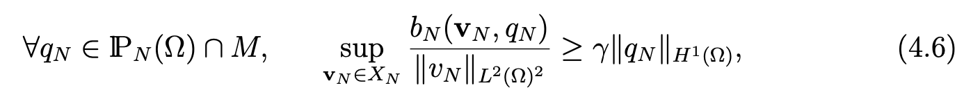
where γ is a positive constant independent from N , by taking vN = ∇qN . Hence, we derive the following theorem.
Theorem 4.1Let f be in C0(Ω)2. Then problem (4.3), (4.4) has a unique solution (uN, pN ) satisfying

Next, we establish a theorem which implies the convergence of our discretization method.
Theorem 4.2Assume that the solution (u, p) of problem (4.3), (4.4) belongs to Hs(Ω)2 × Hs+1(Ω), s ≥ 0, and the data f belongs to Hσ(Ω)2, σ > 1, where Hs(Ω), for non-integral values of s, is defined in (2.1). Then, the following estimate holds

Proof. From the abstract error estimate for the approximation of saddle-point problems (see [7, Chap. IV]), we derive the following estimate:
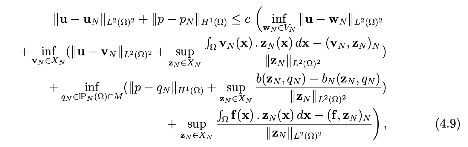
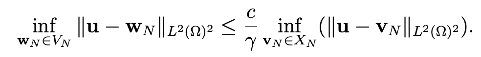
where VN is defined by

Moreover, we recall (see [11, Chap. II, (1.16)]) that
Hence, we derive that, for all vN−1 and fN−1 in lPN−1(Ω)2 and all qN−1 ∈ lPN−1(Ω) ∩ M,

Then, we choose vN−1 = II N−1u (resp. fN−1= IIN−1f), that is to say the orthogonal projection of u (resp. f) on lPN-1(Ω)2 in L2(Ω)2 and qN-1 = II1,Γ2N-1p, where II1,Γ2 N-1p is the orthogonal projection of p on lPN−1(Ω) ∩ M in H1(Ω). It remains to prove the estimate, for any m ≥ 1,

On the one hand, this result is obvious for m = 1. On the other hand, for m ≥ 2, we have (see [7, Chap. III]),
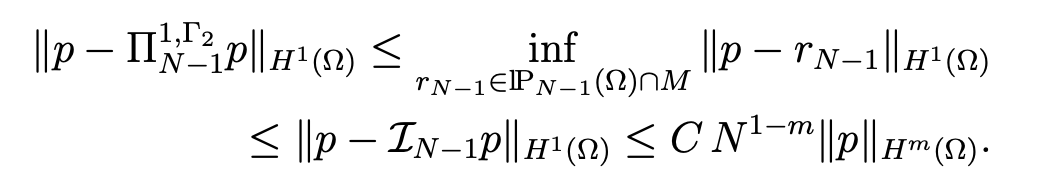
Then, an interpolation argument (see [11, TH 1.4, page 6]) gives (4.11). Finally, the result follows from (4.10), (4.11) and the classic estimate for the orthogonal projection on lPN−1(Ω) in L2(Ω).
Remark 4.3 With the choice XN = lPN(Ω)2, problem (4.3, (4.4) can be interpreted as a collocation scheme. Indeed, by integrating by parts in the discrete bilinear form bN with respect to one of the two variables for each of the two terms of bN (this process being allowed by the precision of the quadrature rule), and choosing as test functions the Lagrange polynomials associated with the grid points of ΞN, it is easily seen that (4.3), (4.4) is equivalent to these to set of equations for uN in lPN(Ω)2 and pN in lPN(Ω) ∩ M:
Second spectral discretization
In order to improve the approximation of the condition div u = 0, we can try to decrease the dimension of the space XN . So, we choose

We note that, in this case the forms b(., .) and bN (., .) are equal on XN × lPN (Ω). It does not appear spurious modes for the pressure, as we can see in the following lemma.
Lemma 4.4 Let ZN be the space

Then ZN = {0}.
Proof. Let qN be in ZN . Since ∂qN/∂x is a polynomial of degree ≤ N − 1 with respect to x, which is orthogonal to lPN−1(Ω), we can write:
with αN and βN in lPN (Ω). In the same way with y in place of x, we have:
with γN and δN in lPN (Ω). Hence, we derive
where λ and μ are real numbers. But, since LN (1) = 0, the condition:
implies λ = μ = 0.
We have to study the following discrete problem:
Find uN in lPN−1(Ω)2 and pN in lPN(Ω)∩M such that


For the inf-sup condition, the choice vN = ∇qN is no longer available, since vN must be in lPN−1(Ω)2. In fact, in the next lemma, we find a inf-sup constant depending on N.
Lemma 4.5 There exists a constant c > 0 independent on N such that

On the one hand, we note that
where aN is a polynomial of degree ≤ N=−1. Then, we have
which implies, using (2.7) and the inverse inequality (2.10),

On the other hand, in view of (2.8), we can write

where rN (x, y) is a polynomial of lPN (Ω) of degree < N − 1 with respect to y. The orthogonality properties imply
By combining this inequality with (4.18), we obtain
In the same way, we have the analogous inequality for ∂q*N/∂y . Thus, we obtain

Next, the equality (4.16) yields

which implies, owing to (2.7) and (2.9),
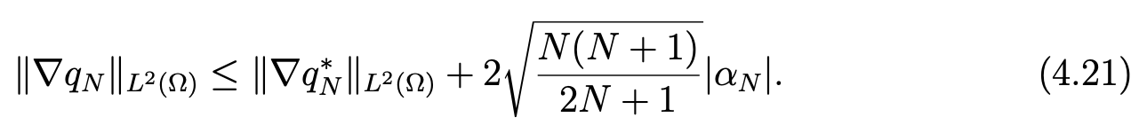
It remains to estimate |αN |. First, we have, owing to (4.16),
But, ∀y ∈ [−1, 1], qN (1, y) = 0, which implies

If we set  , we derive
and, therefore, thanks to a discrete Cauchy-Schwarz inequality
Then, in view of (4.19), we obtain
Finally, (4.20), (4.21) and (4.22) yield
which, in view of (4.17), ends the proof.
The bilinear form (.,.)N and b(.,.) satisfy Brezzi’s conditions with respect to lPN−1(Ω)2 and lPN (Ω) ∩ M (the bilinear form (., .)N is continuous on lPN −1 (Ω)2 and elliptic on lPN−1(Ω), the bilinear form b(.,.) is continuous on lPN−1(Ω) × (lPN(Ω) ∩ M) and verifies the “ inf-sup condition”), see [7, Theorem 2.3, pages 116,117], whence the theorem.
Theorem 4.6Let f be in C 0 (Ω)2 . Then problem (4.13), (4.14) has a unique solution (uN , pN ) satisfying

We establish the convergence of this second discretization in the following theorem.
Theorem 4.7Assume that the solution (u, p) of problem (4.13), (4.14) belongs to Hs(Ω)2 × Hs+1(Ω), s ≥ 0, and the data f belongs to Hσ(Ω)2, σ > 1. Then, the following estimate holds

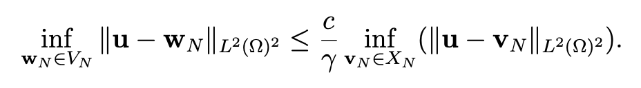
Proof. The abstract error estimate, analogous to (4.39) but with much simplification because of the exactness of the quadrature formulas, yields


where VN is now the space

It remains to estimate the term ∥u − wN ∥L2(Ω)2 . Since u is such that div u = 0 and u . n|Γ1 = 0, there exist a unique ψ in H1(Ω) (see [11, Chap. I and 4]) such that
u = curl ψ and ψ = 0 on Γ1.
Moreover, if u belongs to Hs(Ω)2, we have ∥ψ∥Hs+1(Ω) ≤ c∥u∥Hs(Ω)2. Let us define the operator π ̃N1 (see [7, Chap. II]) on H1(Λ) by

where the function φ ̃ stands for
Note that the definition of π ̃1N is available, because φ ̃ belongs to H10(Λ), and that π1,0Nφ ̃ and φ coincide in −1 and 1. In [8, Section 7], the following estimate is proven, for all r ≥ 1 and all function φ in Hr(Λ):

Assuming s ≥ 1, we set
Since  we can verify that RN−1 (u) belongs to VN and, in view of (4.26), that
Finally, we derive, for s ≥ 1,

Since we have an interpolation argument gives the result of approximation in VN for any s ≥ 0 and the estimate of the theorem follows.
Third spectral discretization
The third discretization comes from the variational formulation (3.13), (3.14). We define the space XN by

Let MN be a subspace of lPN( Ω) that we shall set later. Then, we consider the following discrete problem:
Find uN in XNand pN in MN such that


where the form b∗N is define by

In order to choose MN , we begin to identify the spurious modes for the pressure. These spurious modes for the pressure are derived by elimination from those of classic Stokes problem (see [7, Chap. IV]). In particular, we can verify: ∀vN ∈ XN , b∗N (vN , qN ) = 0, for qN (x, y) = LN (x) or LN (x)LN (y). We obtain the following lemma.
Lemma 4.8 Let ZN∗ be the space

Then ZN∗ is spanned by (LN (x), LN (x)LN (y)).
Finally, let MN stand for the orthogonal complement of ZN∗ for the scalar product in L2(Ω) or for the scalar product (.,.)N, owing to (2.11). The inf-sup condition is given in the next lemma.
Lemma 4.9There exists a constant c > 0 independent from N such that
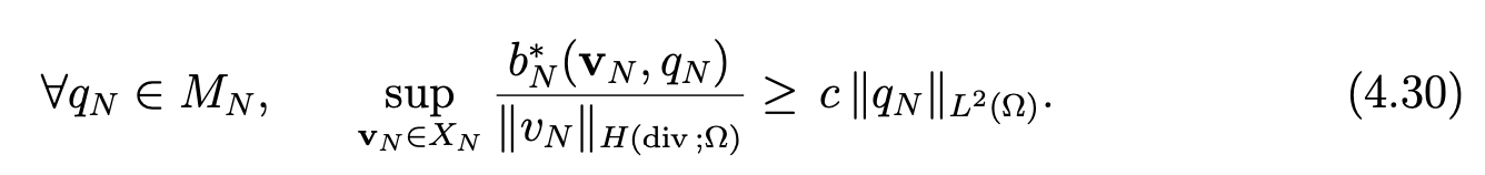
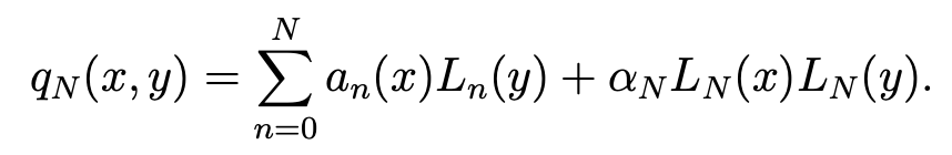
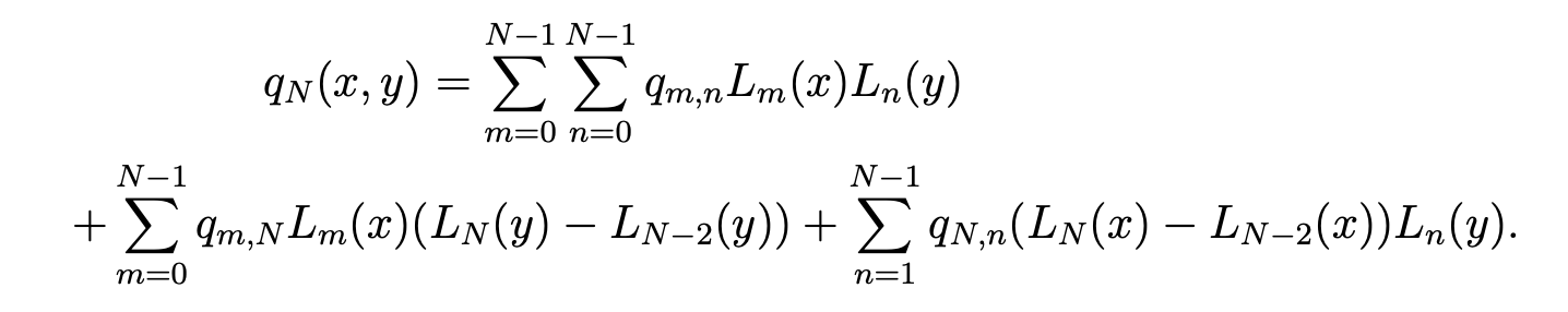
Proof. Any function qN in MNhas the expansion
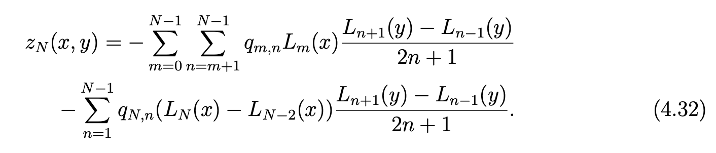
With the convention L−1 = 0, we choose wN = (wN , zN ) with
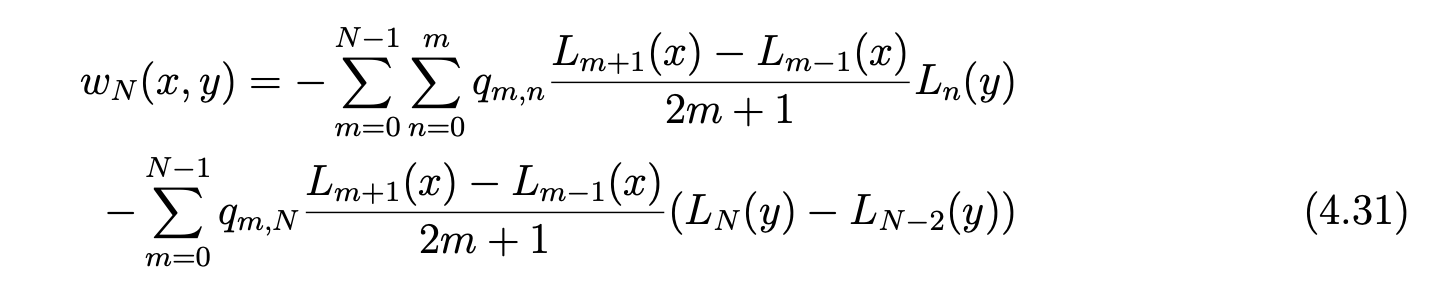
and
Then, in view of (2.8), we have

since wN .n|Γ1 = zN|Γ1 =0. As in[6,Chap. IV], we prove
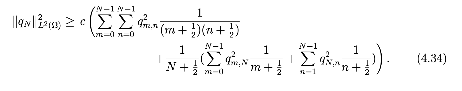
Hence, we derive, in the same way as in [8, Section 24]
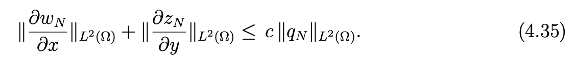
Next, setting wN∗ (x, y) = wN (x, y) − q0,0L1(x) − q0,N L1(x)(LN (y) − LN−2(y)), we note that wN∗ (±1,y) = 0 for −1 ≤ y ≤ 1. Then, the Poincar ́e-Friedrichs inequality, applied with respect to x or y, yields

Hence, owing to (4.35) and the estimate
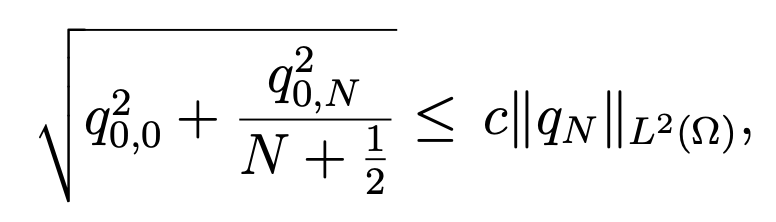
which is derived from (4.34), we obtain

Finally (4.35) and (4.36) imply
and, in view of (4.33), the choice vN = wN in b∗N (vN , qN ) is available and gives the inf-sup condition (4.30).
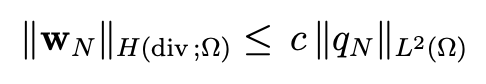
From the previous lemma, we derive the following theorem.
Theorem 4.10Let f be in C0(Ω)2. Then problem (4.27), (4.28) has a unique solution (uN , pN ) satisfying

Sketch of the proof. From(4.27), we derive (uN , uN )N = (LNf , uN )N . Then, Owing to div uN = 0 and (2.13), we derive ∥uN ∥H (div ;Ω) ≤ 3∥LNf ∥L2 (Ω) . Next, the inf-sup condition (4.30) and (4.27) imply
Hence, in view of (2.13), we obtain
which ends the proof.
Next, in the same way as in Theorem 4.2, we prove an optimal error estimate.
Theorem 4.11 Assume that the solution (u,p) of problem (4.27), (4.28) belongs to Hs(Ω)2 ×Hs(Ω), s ≥ 0, and the data f belongs to Hσ(Ω)2, σ > 1. Then, the following estimate holds.

Sketch of the proof. Again, from the abstract error estimate for the approximation of saddle-point problems (see [7, Chap. IV]), we derive the following estimate:
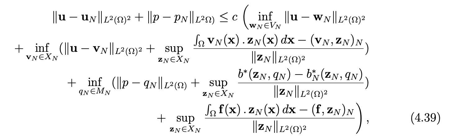
where VN is defined by
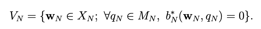
Moreover, we still have (see [11, CH. II, (1.16)])
We end the proof in the same way as in Theorem 4.2.
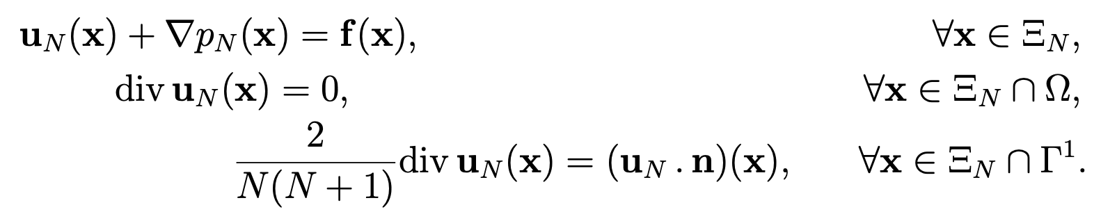
Remark 4.12 As for the first discretization, problem (4.27, (4.28) can be interpreted as a collocation scheme. In the same way, we prove that (4.27), (4.28) is equivalent to the set of equations for uN in XN and pN in MN:
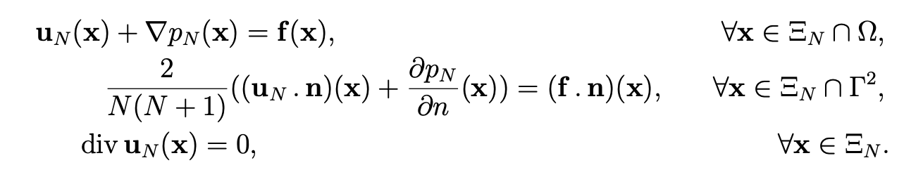
Therefore, the discrete solution uN is exactly divergence-free, which is important for some applications.
Numerical Results
The convergence of the methods corresponding to the first and third discretizations were tested in a problem of the type (1.1)-(1.4), with homogeneous boundary conditions. Precisely, we tested the convergence of these methods to the exact solution u(x,y) = (πx2 cos(πy), −2x sin(πy) and p(x, y) = y sin(πx), which means that we studied the convergence of these methods for Problem (1.1)-(1.4), with

and homogeneous boundary conditions. In addition, we tested the convergence to 0 of the divergence for both methods.
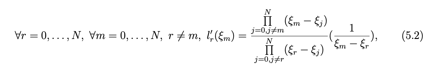
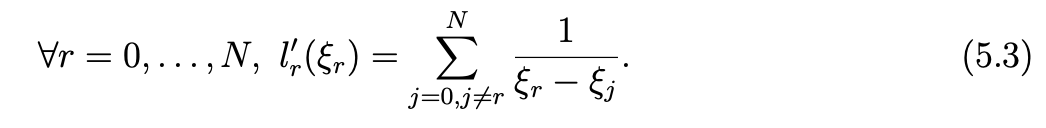
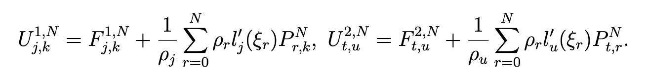
We shall use the Lagrange polynomials. We denote lr the Lagrange polynomial associated to the Gauss-Lobatto point ξr, 0 ≤ r ≤ N, the expression of which is
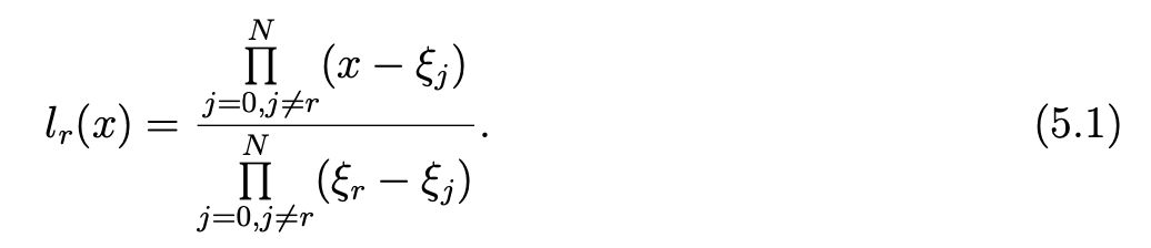
The derivative lr′ verifies the following equalities
Uzawa's algorithm
Problem (4.3), (4.4), Problem (4.13), (4.14) and Problem (4.27), (4.28) are equivalent to a linear system of the type :
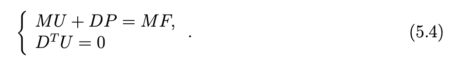
The unkowns are the vectors U and P which represent respectively the velocity and the pressure values on a given grid points. The data f is representated by the vector F on the same grid points. The diagonal matrix M is the weight matrix, while the matrix D is associated to the form bN for the first and second spectral discretizations and to the form b∗N for the third spectral discretization and DT is the transposed matrix of D.
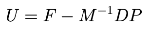
Uzawa’s algorithm consists in rewriting the first equation of system (5.4) as: U = F − M−1DP and substituting in the second equation. We obtain a new equation for the pressure P:

Next, we solve this symetric system either directly if the matrix DT M−1D is invertible or by diagonalizing the matrix DTM−1D if not, because the spurious modes correspond to eigenvalues of the matrix equal to zero. Next, we compute the velocity via the formula
and its divergence by multiplying U on the left by the matrix DT . Finally, we test the convergence to 0 of its divergence.
Implementation of the rst discretization
We take (lj(x)lk(y),0), (0,lj(x)lk(y)), 0 ≤ i,j ≤ N as a basis of XN and
lr(x)ls(y),1≤r≤N−1,0≤s≤N as a basis of PN(Ω)∩M. The unknowns are
the velocity uN = (u1N,u2N) and the pressure pN. For j = 1,2, for 0 ≤ r,s ≤ N, we
denote ,where f=(f1,f2) represents the data, and, for 1≤r≤N−1, for 0≤s≤N, we denote PNr,s=pN (ξr,ξs). So, we have

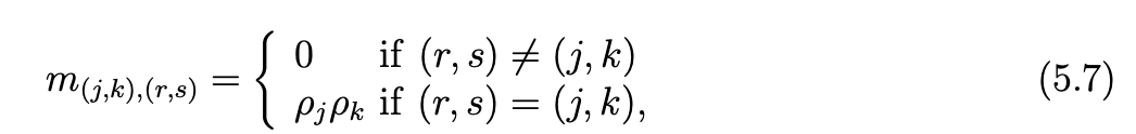
Let us define the (N + 1)2 × (N + 1)2 diagonal matrix 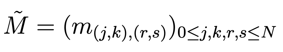 with
with
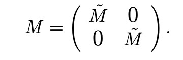
and the 2(N + 1)2 × 2(N + 1)2 diagonal matrix
By setting vN(x,y) = (lj(x)lk(y),0), for 0 ≤ j,k ≤ N and, next, vN(x,y) = (0,lj(x)lk(y) in (4.3), (4.4), we obtain the matrix system (5.4) where the column matrices U, P and F are defined by
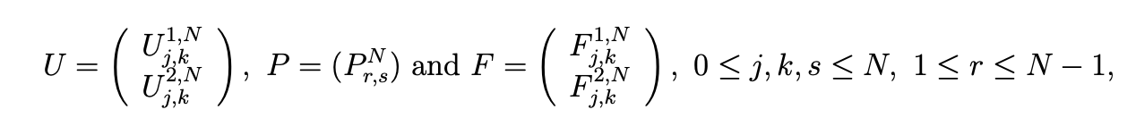
and, with (.,.)N defined by (4.1), the 2(N +1)2 ×(N2 −1) matrix D by

where (j, k) represents the row index, (r, s) the column index, 0 ≤ i, j, s ≤ N , 1≤r≤N−1, for the matrices D1,N and D2,N. Note that U and F are 2(N+1)2×1 matrices and P is a (N2 − 1) × 1 matrix.
Proposition 5.1 The (N2 − 1) × (N2 − 1) square matrix DT M−1D is invertible.
Proof. We just have to prove that the rank of the matrix D is N2 − 1. Let us assume that the rank of the matrix D is strictly smaller than N2 − 1. Then, there exist a sequence of real number (qr,s),1≤r≤N−1,0≤s≤N, where all the real numbers qr,s are not equal to zero, such that
where Dr,s are the column vectors of the matrix D. Setting  the previous equality is equivalent to
which is in contradiction with the property that there is no spurious mode.
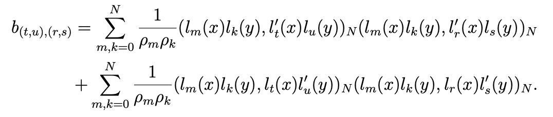
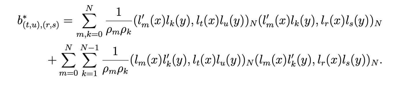
We have to compute the matrix DTM−1D = (b(t,u),(r,s)), 1 ≤ r, t ≤ N −1, 0 ≤ s, u ≤ N.
Owing to the previous expression of the matrices D and M, we obtain
Next, we change the numbering for the matrix DT M−1D. Let us define the mapping φ by

Note that φ is a one to one mapping from {1,...,N −1}×{0,...,N} to {1,...,N2 −1} and we note

Note that ψ1(i)-1 and ψ2(i) are respectively the quotient and the remainder of the euclidian division of i − 1 by N + 1. Then, we can denote

where (t, u) = (ψ1(i), ψ2(i)) and (r, s) = (ψ1(j), ψ2(j)).
Computing the elements ai,j of the matrix DTM−1D yields
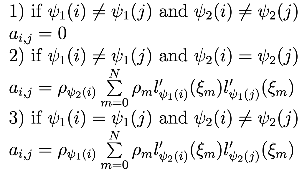
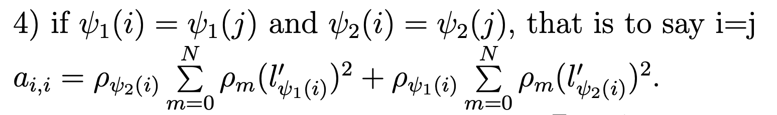
Thus, most of elements of the matrix DT M−1D are equal to zero.
Next, we determine the column matrix DT F = (ci,1) by

Hence, owing to (5.2) and (5.3), we compute the list [lk′(ξm), 0 ≤ k,m ≤ N], which allows us to determine the elements of the matrices DT M−1D and DT F. Since the matrix DT M−1D is invertible, the equation (DT M−1D)X = DT F has a unique solution X. Then we derive easily the column matrix P =(PNr,s)such that PNr,s =Xφ(r,s) ,1≤r≤N−1, 0 ≤ s ≤ N and, next, the column matrix U, thanks to the relation U = F − M−1DP. Setting PN0,t = PNN,t = 0 for 0 ≤ t ≤ N in accordance with the boundary conditions, we obtain
Finally, we derive
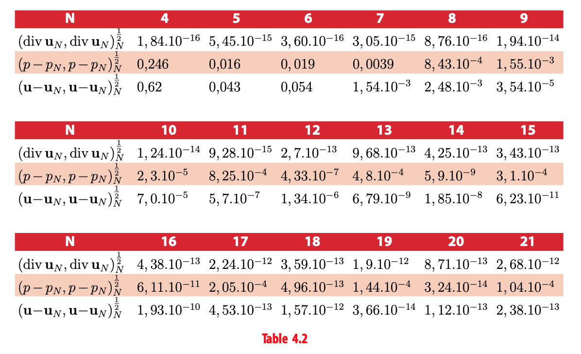
We give the values of (div uN, div uN)N1/2 , (p−pN,p−pN)N1/2 and (u−uN,u−uN)N1/2 for N between 4 and 21.
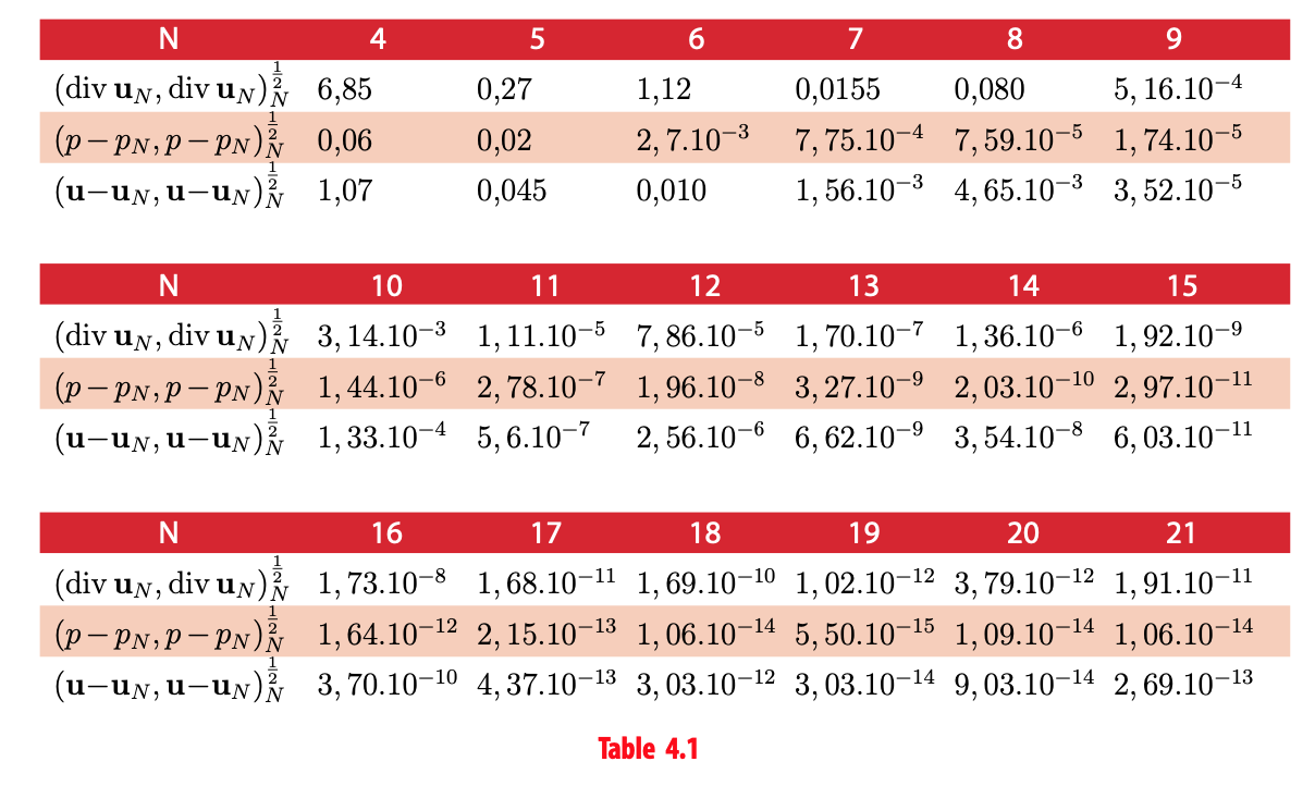
We shall comment these results on comparing them with these ones of the third discretization.
Implementation of the first discretization
We only sketch the method because the first and third discretizations are rather similar, but we shall point out the differences between both discretizations.
First, the space XN is not the same, because boundary conditions are taken in account. Thus, we take (lj(x)lk(y),0), (0,ls(x)lr(y)), 0 ≤ i,j,s ≤ N, 1 ≤ r ≤ N − 1 as a basis of XN.
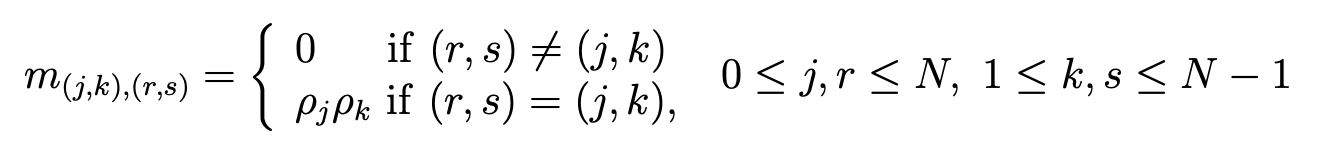
Second, we shall compute the pressure pN as the orthogonal projection on MN of an element of lPN(Ω) and we take lr(x)ls(y), 0 ≤ r,s ≤ N as a basis of lPN(Ω). For 0 ≤ r,s ≤ N, we denote U1,Nr,s =u1N (ξr,ξs),PNr,s =pN(ξr,ξs) and for 0≤r≤N,1≤s≤N−1, we denote U2,Nr,s = u2N (ξr ,ξs ). Let us define the matrix M ̃1 = M ̃, where M ̃ is given by (5.7), the(N2 −1)×(N2 −1)matrix M ̃2 =(m(j,k),(r,s)) with
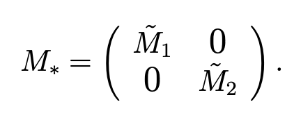
and the 2N(N + 1) × 2N(N + 1) diagonal matrix
In the same way as the first discretization, we derive the following matrix system
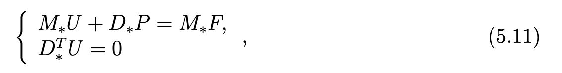
where the column matrices U, P and F are defined by

and the 2N(N +1)×(N +1)2 matrix D∗ by

We have to compute the matrix DT∗M−1∗D∗ =(b∗ (t,u),(r,s) ),0≤r,s,t,u≤N. In the same way as the first discretization, we obtain
Next, as in the first discretization, we change the numbering for the matrix DT∗M−1 ∗D∗. Let us define the mapping φ∗ by

Note that φ∗ is a one to one mapping from {0,...,N}2 to {1,...,(N +1)2} and we note

Note that ψ1∗(i) and ψ2∗(i) are respectively the quotient and the remainder of the euclidian division of i−1 by N +1. Then, we can denote

where (t, u) = (ψ1∗(i), ψ2∗(i)) and (r, s) = (ψ1∗(j), ψ2∗(j)).
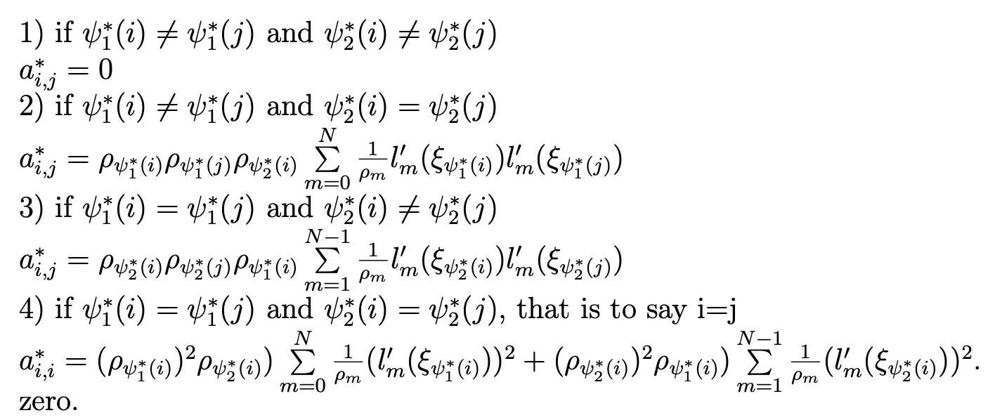
Computing the elements a∗i,j of the matrix DT∗ M−1∗D∗ yields
Next, we determine the column matrix D∗T F = (c∗i,1) by

Now, we deal with the main difference between both discretizations. In the third discretization, the matrix DT*M-1*D* is not invertible and the computation of the pressure is more complicated. First, let  be a spurious mode, that is to say
an element of the space ZN∗ defined in Lemma 4.8. In the same way as in the proof of
Proposition 5.1, considering that the matrices DT*M−1*D* and D* have the same rank, we
obtain the following equivalences
be a spurious mode, that is to say
an element of the space ZN∗ defined in Lemma 4.8. In the same way as in the proof of
Proposition 5.1, considering that the matrices DT*M−1*D* and D* have the same rank, we
obtain the following equivalences

where Q is the column vector (q t,u) 0≤t,u≤N . We can consider the matrix DT*M−1*D* as the matrix of a linear mapping f from the vector space lPN(Ω) into itself equipped with the basis B = (li(x)lj(y))0≤i,j≤N .Therefore, ZN∗ is the eigenspace associated to the eigenvalue equal to 0 of the linear mapping f or, equivalently, of its matrix DT*M−1*D* . Note that this basis is orthonormal for the scalar product (.,.)N. We can diagonalize the positive symmetric matrix DT*M−1*D* and, thus, there exist a diagonal matrix Λ and an orthogonal matrix R such that DT∗ M-1∗ D∗ = RΛR-1 and such that the diagonal elements of Λ, that is to say (λi,i)1≤i≤(N+1)2 are in increasing order. Note that the matrix Λ is the matrix of f in a basis B′ = (hi)1≤i≤(N+1)2 of lPN (Ω), which is orthonormal for the scalar product (., .)N , the elements of which are the eigenvectors of the matrix DT*M−1*D* . Let P′ be the column matrix the elements of which are the components of the pressure pN in the new basis B' of lPN(Ω). We have P′ =RTP =R−1P and the following equivalence

Since ZN∗ is a two dimensions space, B0′ = (h1 , h2 ) is the basis of ZN∗ and (hi )3≤i≤(N +1)2 is a basis of MN = (ZN∗ )⊥. Therefore, we determine the column vectors P′ and P by

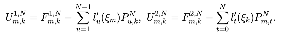
and we have  In the same way as for the first discretization, we derive the column matrix U by the relation U = F − M−1*D*P, which gives, for
0 ≤ j, k, t ≤ N , 1 ≤ u ≤ N − 1,
In the same way as for the first discretization, we derive the column matrix U by the relation U = F − M−1*D*P, which gives, for
0 ≤ j, k, t ≤ N , 1 ≤ u ≤ N − 1,
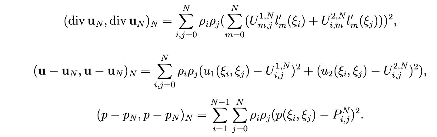
Finally, considering the boundary conditions, we set U2,Nt,0 = U2,Nt,N = 0, 0≤t≤N , and we obtain the same formulas as in the first discretization for (div uN , div uN)N , (u − uN , u − uN)N and (p - pN, p - pN)N . We also give the values of ( div uN , div uN )N1/2 , (p−pN ,p−pN)N1/2 and (u- uN, u - uN)N1/2 for N between 4 and 21.
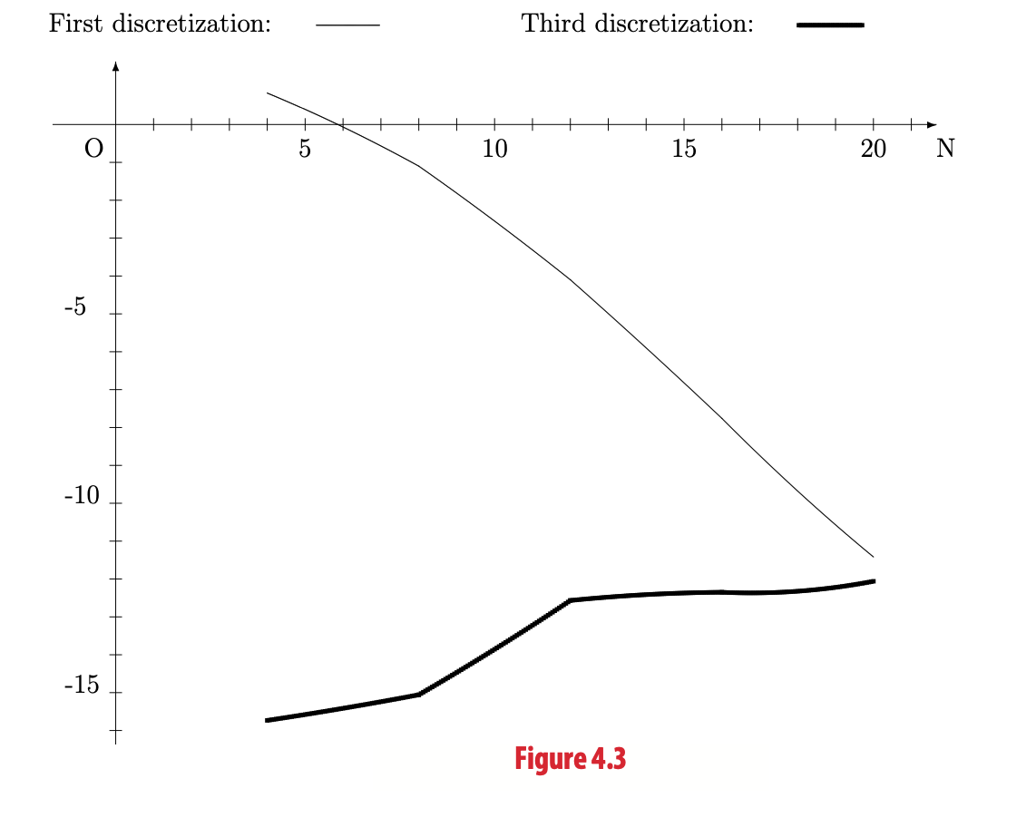
Logarithm to the basis 10 of (div uN , div uN )N1/2in function of N for the first and third discretizations
Conclusion
Continuous problem and discretizations
We studied the Darcy problem by defining two equivalent variational formulations corresponding to two different bilinear forms b and b∗. The first one requests a more regular pressure, which is bounded in H1(Ω). The second one is less classic and was introduced by A. Quarteroni and A. Valli (see [14]). This second variational formulation is important because it allowed us to constuct a spectral method which gives a divergence-free discrete solution.
Moreover, by studying a mixed problem of Dirichlet-Neumann for the Laplace operator, we proved regularity results with the solution (u,p) in H1(Ω)2 ×H2(Ω) as long as the data is regular enough.
The first variational formulation led us to two spectral discretizations. In the first one, the discrete solution is not divergence-free, which is a disadvantage for some applications. However, we obtain a fully optimal error estimate for the velocity and the pressure. In the second discretization, it does not appear spurious modes for the pressure. Moreover, because of the exactness of the quadrature formulas, the error estimate is easier to obtain. However, the error estimate for the pressure is not optimal, because the inf-sup constant depends on N.
The second variational formulation led to a third spectral discretization. There are spurious modes, which complicate the study, but the discrete velocity is divergence-free, which is important when the system is a stage of solving of a time-dependent problem, and the error estimate for the velocity and the pressure is fully optimal. In conclusion, this third discretization is the best discretization and we will only use it hereafter.
Comparison of both spectral discretizations
Tables 4.1 and 4.2 test the convergence of respectively the first and third discretizations to the exact solutions. For the first discretization, we see the convergence to zero of (div uN, div uN)N1/2 , about 10−1 for N = 8 and about 10−12 for N = 19. Concerning the third discretization, we see that the quantity (div uN , div uN )N1/2 is very small for all values of N, about 10−16 for N = 4 and about 10−12 for N = 20. Thus, we verify that, in the third discretization, the discrete solution uN is exactly divergence-free, which is important, as we saw previously. This property appears clearly in Figure 4.3, which represents the logarithm to the basis 10 of the quantity (div uN , div uN )N1/2 as a function of N , for even N from 4 to 20, for both discretizations.
Regarding the velocity, the discrete solution uN converges fast to the exact solution u for both discretizations. For the pressure, we also obtain fast convergence, except for odd N in the third discretization.
References
Achdou, Y., Bernardi, C. & Coquel, F. “A priori a posteriori analysis of finite volume discretizations of Darcy’s equations”, Numer. Math. 96 (2003), 17-42.
Azaïez, M., Bernardi, C. & Grundmann, M. “Méthodes spectrales pour les équations du milieu poreux”, East West Journal of Numerical Analysis, No. 2, 1994.
Babuska, I. "The finite element method with lagrangian multipliers”, Numer. Math. 20, pp. 179-192 (1973).
Bègue, C., Conca, C., Murat, F. & Pironneau, O. “Les équations de Stokes et de Navier-Stokes avec des conditions aux limites sur la pression”, Nonlinear Partial Differen- tial Equations and their Applications, Coll'ege de France Seminar, vol. IX (1988).
Bernard, J.M. "Spectral discretizations of the Stokes equations with non standard boundary conditions”, Journal of Scientific Computing, 20(3), 355-377 (2004).
Bernardi, C., Canuto, C. & Maday, Y. "Spectral approximations of the Stokes equa- tions with boundary conditions on the pressure”, SIAM J. Numer. Anal. 28, No 2 (1991), p. 333-362.
Bernardi, C. & Maday, Y. Approximations spectrales de problèmes aux limites ellip- tiques, Springer-Verlag, Paris, 1992.
Bernardi, C. & Maday, Y. Spectral Methods, Handbook of Numerical Analysis, Vol. V, Paris (1997).
Brezzi, F. "On the existence, uniqueness and approximation of saddle-point problems arising from Lagrange multipliers”, R.A.I.R.O., Anal. Mumer. R2, PP. 129-151 (1974).
Chorin, A.J. " Numerical solution of the Navier-Stokes equations”, Math. Comput. 22 (1968), 745-762.
Girault, V. & Raviart, P. A. Finite Element Methods for Navier-Stokes Equations,Springer-Verlag, Berlin (1986).
Grisvard, P. "Elliptic Problems in Nonsmooth Domains”, Pitman Monographs and Studies in Mathematics, 24, Boston (1985).
Necas, J. les Méthodes Directes en Théorie des Equations Elliptiques, Masson, Paris (1967).
Quarteroni, A. & Valli, A. Domain decomposition methods for partial differential equations, Oxford science publication (1999).
Temam, R. "Une méthode d’approximation de la solution des équations de Navier- Stokes”, Bull. Soc. Math. France 98 (1968), 115-152.