

Labor displacement effects over inter-temporal earnings mobility
Efectos intertemporales del desplazamiento laboral sobre la movilidad de ingresos
ACI Avances en Ciencias e Ingenierías
Universidad San Francisco de Quito, Ecuador
Received: 15 May 2021
Accepted: 26 January 2022
Abstract: I study how involuntary job loss affects workers’ inter-temporal labor earnings mobility. I use Panel Study Income Dynamics (PSID) 1973-2017 survey waves to construct transition probability matrices and compute ordered logistic regression estimates. I find that being displaced increases downward mobility compared to never displaced workers. The reduction of hours worked, large spells of unemployment and the destruction of firmspecific human capital depreciate the market value of a displaced worker generating significant labor income losses.
Keywords: PSID, displacement, involuntary job loss, inter-generational mobility, income mobility, labor economics.
Resumen: En este trabajo, yo estudio cómo una separación laboral involuntaria afecta a la movilidad intertemporal en la distribución de ingresos laborales de los trabajadores. Con ese fin, uso datos de Panel Study Income Dynamics (PSID) de los años 1973-2017 para construir matrices de probabilidad de transiciones y para obtener estimadores a través de una regresión logística ordenada. Encontré que estar desplazado laboralmente aumenta la probabilidad de que el trabajador esté en deciles de ingreso inferiores en contraste a los resultados de un trabajador que nunca ha experimentado desplazamiento. La reducción de horas trabajadas, largos períodos de desempleo y la destrucción de capital humano específico deprecian el valor de mercado de un trabajador desplazado, así se generan perdidas de ingreso significativas.
Palabras clave: PSID, desplazamiento laboral, movilidad intergeneracional, movilidad de ingresos, economía laboral.
INTRODUCTION
From 1973 to 2017, nearly 14% of workers have experienced displacement in the United States. After two years of involuntary job loss, displaced workers perceive, on average, $14,622 real1 labor earnings while never displaced individuals earn $27,388. This significant gap shows the importance of being aware of how displacement influences movements throughout the labor income distribution and its implications for policies designed to mitigate the adverse effects of unemployment. With this in mind, how do displacement affect long-term income mobility?
To answer this question, I use the 1973-2017 survey waves of the Panel Study Income Dynamics (PSID) to analyze how involuntary job loss affects workers’ inter-temporal labor earnings mobility across time. To study the impact of displacement, I construct transition probabilities to compare mobility patterns among displacement status. Furthermore, I use an ordered logistic regression to estimate the long-term income loss of displaced individuals. Then, I use these estimates to calculate the probability of a displaced worker being in any decile of the income distribution relative to never displaced workers. The increased probability of moving downward after displacement occurs because displacement alters the labor income by decreasing hours worked, causing spells of unemployment, and possibly destroying the human capital formation.
I contribute to the existing literature on labor displacement in two ways. First, by extending the time horizon for the analysis, I show that displacement adverse effects are more severe two years after displacement increasing the probability of being at the bottom halfofthe labor income distribution by 135% in contrast to the probability in the year of displacement. Second, by using transition matrices and ordered logistic regression, I can compare mobility over displaced and never displaced workers considering the effects of specific demographic traits. The pre-displacement income gap is significant in the transition matrices where I do not control for individual characteristics. Also, the postdisplacement gap tends to close faster when I control for specific workers’ attributes.
Literature on the effects of involuntary job losses begins with magnitude estimations of income losses [1, 2, 3]. It has also been done using large data sets like the PSID [4, 5, 6, 7, 8]. Also, a compact summary of the main results across several data sets can be found [9].
Another approach taken in the literature is the study of trends upon job losses [10] and the persistence of its adverse effects [5]. Some have explained these losses using a displacement typology [11] and demographic traits [12]. Also, some explanations for the variations on the empirical results are labor market conditions [13], losses in firm wage premiums [14], idiosyncratic ability [15], and transferability of human capital across occupations [16].
Nevertheless, there is little literature that focus on mobility and displacement. A study finds an increase of the proportion of workers with earnings below than $10,000 due to displacement [7], while other use probit models to explore how voluntary and involuntary job losses affect mobility. On the other hand [8], another finds that the probability of entering poverty increases due to displacement [17]. This goes in line with Jolly, where he finds that the probability of being at the bottom half of the earnings distribution increases significantly, not only in the year of displacement, but also several years after. Furthermore, he considers additional measures of financial well-being that reduce the short and long-term impact of displacement [6].
This paper is organized as follows. Section two presents the methodology. In Section three, I describe the data. Then, Section four provides the results, and Section five concludes and provides a brief discussion on further steps to study the long-term effects of job displacement.
METHODOLOGY
My primary goal is to study the effects of job displacement on an individual’s movement over the ranking in labor income distributions. For this reason, this analysis uses two methodologies: transition matrices and ordered logistic regression. Each approach observes how displacement affects income mobility over time. The first provides a brief overview of the probability of workers’ movements across the distribution and gives information about the persistence of income shocks. The second approach permits the identification of factors that influence the workers’ movement throughout income deciles.
Transition matrices
Transition matrices estimate the probability of specific movements across the distribution over time. They also provide information about the persistence of income shocks, allowing to observe if the negative shock of being displaced is persistent or not. On the one hand, if the shock is persistent, the probability of moving between deciles will increase. On the other hand, if the shock is transitory, the probability of changing income deciles will be the same in the short and long run. The first step to build transition matrices is to generate labor income deciles over the sample’s distribution. This procedure maintains the upper and lower distribution bounds fixed over the estimations. Later on, it is necessary to split the sample among displaced and never displaced individuals to identify their differences.
This section uses the same notation and methodology as Jolly [6]. It starts with the formulation of binary variables that capture movements across deciles for every individual of each data subset. I follow each transition by the indicator which is equal to one if the individual i moves from decile d to decile I between periods t and t + r. Then, I create new variables and calculate their mean according to the movements’ direction and magnitude. For example, the variable upward 8 refers to the sum’s average of individuals’ movements from decile one to decile nine and decile two to decile ten.
The reference point t differs from each data subset. On the one hand, the displaced workers’ reference period is four years before the job loss, ensuring previous labor market attachment. On the other hand, the reference point for the never displaced comes from a random number among periods that follow a uniform distribution.
Ordered Logistic Regression
An ordered logistic regression gives more accurate results than transition matrices. Including control variables allows a more profound understanding of how different demographic factors influence displacement adverse effects. Its construction begins by estimating an earnings equation using a fixed-effects estimator to observe the process of wage determination. This data then allows the computation of income deciles given the parameter estimates distribution. Furthermore, I use an ordered logistic regression where the estimated deciles are the dependent variable. Each outcome’s marginal effects represent the probability of being at any decile in a specific period.
The earnings equation (1) is similar to the one used by Couch [9]:
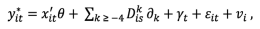 (1)
(1)where xit includes demographic characteristics of the sample and quadratic potential experience, and θ captures the effect of these traits. In addition, a dummy variable equal to one if the individual experiments displacement in year s and k indexes these variables four years before the job loss. Also, γt are the period dummy variables and is the time-variant error. Finally, it is assumed that vi is the time-invariant and unobserved individual effect, and it has independence of the observed predictor variables. The latter are independently and randomly distributed as normal with mean zero and known variances, and respectively.
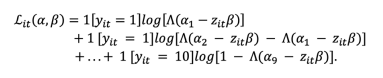
The individual i falls in one of the following categories, where αjs are the lower and upper bounds of each decile:
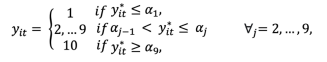 (2)
(2)To obtain the probability that yit takes in each decile, I use an ordered logistic regression. To simplify notation, I assume:
 (3)
(3)
 (4)
(4)and, after rearranging, I obtain:
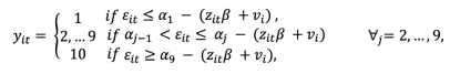 (5)
(5)The probability of each case is easy to obtain due to the normal distribution assumption on and vi. It goes as follows:
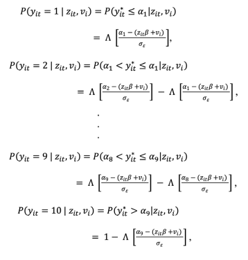 (6)
(6)where the parameters α and β are estimated through the log-likelihood function:
 (7)
(7)Since β’s magnitude is not my primary interest, I focus on the outcomes’ marginal effects. These can be obtained by taking the derivative of (6) with respect to xit:
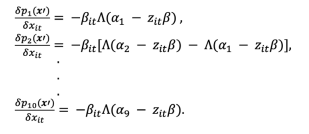 (8)
(8)DATA
I use the Panel Study of Income Dynamics (PSID) of the US. It is currently the most comprehensive longitudinal household survey, starting in 1986 until nowadays. Consequently, it was annually conducted from 1968 to 1997 and biennially thereafter. By these methods, the PSID collects information for 18000 individuals of 5000 families. It covers topics like employment, income, wealth, and expenditures, among others.
I draw on biennial data from 1973 to 2017 to follow individuals over the same time intervals. The subjects of analysis are male heads of households between 25 and 61 years old who reported non-zero labor earnings. I follow these selection criteria to avoid potential biases due to maternity, child-rearing, and retirement.
The household’s heads financial well-being measure is the reported annual labor earnings2 converted to real dollars using the 1982-1984=100 Consumer Price Index. These earnings act as the direct reward of being involved in the labor force. It is crucial to notice that the reported labor earnings refer to the annual’s income of the year before the survey. For that reason, the analysis covers 1972 to 2016 annual labor earnings.
An individual is categorized as displaced when he has experienced involuntary job loss due to plant closure or laid-off. Displacement occurs in the calendar year before the survey wave, and I only follow up the first displacement. All displaced workers must have four consecutive years of positive labor earnings before displacement occurs, to ensure previous labor market attachment. This definition is consistent with the one used by Jolly [6]. The other group subject to analysis are the never displaced individuals. They are the household heads who have never experienced job displacement during those years. Considering these selection rules, 31,688 individuals meet the sample criteria; of this group, 4,460 have experienced displacement between 1973 and 2017.
In the ordered logistic regression, I use specific demographic characteristics like age, race, years of education, the number of children under 18, marital status, blue-collar occupation, manufacturing industry, region of residence, wife’s education, and age. Also, the potential experience equals age minus education minus six. Ifthe individual has less than 12 years of education, then potential experience equals age minus 18. In this way, I avoid the overcompensation of less-educated workers by assigning them larger values of experience. Here education is the same over time, by drawing on each subject the reported education on the most recent survey.
Descriptive statistics
Table 1 displays each sample subgroup’s means and its difference to highlight the main distinctions across groups. The mean of the head’s annual labor income is $12,962 less when the individual experiences displacement than a worker who has never experienced it. It reaffirms the findings of Lachowska where the reduction of work hours almost entirely explains annual earnings losses [10]. Furthermore, displaced individuals tend to be younger and less educated; therefore, they have lower potential experience than never displaced workers. As Addison show, education level and workers’ skills play an essential role in the depth and length of displaced workers’ earning losses [12]. The group subject to analysis tends to have more black people and fewer married individuals. Also, the sample is employed more in blue-collar occupations than in manufacturing industries. This last trait is crucial to understand human capital transferability across occupations and its role in determining post-displacement earnings.
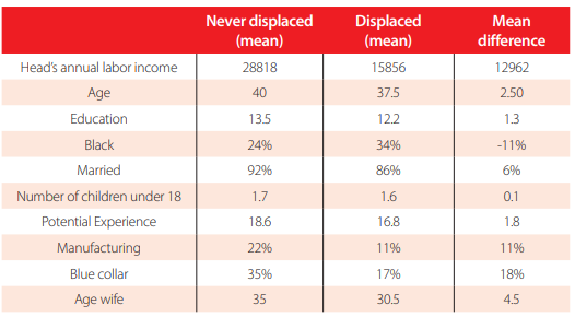
Descriptive Statistics by Displacement Status
Notes: Mean calculations use data from all years per observation.Total number of observations: 528 609 Number of observations if displaced: 9 526 Source: 1973-2017 PSID waves.
RESULTS
Transition matrices
Table 2 indicates transition probabilities by displacement status for labor income of household head. The columns show the relative time changes for never displaced and displaced individuals. For example, column t + 4 specifies the change from the year of displacement to four years after displacement. At the same time, the rows specify the movement made for the individual in a given period. As previously explained, Upward 8 refers to the movement of eight deciles up. Also, the entries in black show the mean differences between displacement status, these are significant at the 5% significance level.
| t-4 | t-2 | t | ||||
| Movement | Never displaced (%) | Displaced (%) | Never displaced (%) | Displaced (%) | Never displaced (%) | Displaced (%) |
| Upward 9 | 0.0886 | 0.0000 | 0.1466 | 0.0000 | 0.0703 | 0.0000 |
| Upward 8 | 0.2444 | 0.0448 | 0.3177 | 0.2242 | 0.2658 | 0.2242 |
| Upward 7 | 0.1497 | 0.0897 | 0.3360 | 0.3812 | 0.7790 | 0.4484 |
| Upward 6 | 0.4613 | 0.8969 | 0.7271 | 0.6278 | 0.9165** | 0.7623** |
| Upward 5 | 1.0692 | 1.2780 | 1.4267** | 0.8744** | 1.6710** | 1.1435** |
| Upward 4 | 1.4664*** | 1.4798*** | 2.4439*** | 1.3677*** | 2.9297*** | 1.8161*** |
| Upward 3 | 3.3879*** | 5.5157*** | 4.8298*** | 3.2287*** | 5.0345*** | 2.6233*** |
| Upward 2 | 6.8491*** | 6.7040*** | 7.8909*** | 5.2691*** | 8.3155*** | 6.7937*** |
Transition matrices
Notes: For the never displaced group, a random starting point is selected, while for the displaced ones, the period t is determined as the year of displacement. The table shows the results of a two-tailed test to determine if the difference among each group is statistically significant.*** p < 0.01, ** p < 0.05, * p < 0.1 Source: 1973-2017 PSID waves.
Four years before displacement, I observe a difference of ten pp. in the probability of maintaining the worker’s position in his income decile. Upward and downward mobility is almost the same for both groups. Nevertheless, downward mobility is more likely to happen when the individual had experienced displacement. This outcome highlights the possible existence of productivity differences before displacement among groups. If future displaced workers have low productivity, it reflects on a proportional decrease in wage. Also, it explains the tendency to move to a lower income decile instead of keeping their income distribution position.
Two years before displacement, the immobile gap becomes shorter, and downward mobility tendency remains the same. Comparing results from four to two years before displacement, the probability of moving downward rises. It points out productivity differences among displacement status. Furthermore, a repeated decrease of the annual labor earnings acts as a sign of the less productive time. The latter can result in workers being laid-off due to the inability to increase their productive time or a general decrease in the enterprise’s production, leading to a plant closure.
In the year of displacement, there is a notorious difference in the mobility probabilities. The probability of keeping the deciles position is 12 pp. less when the worker had experienced displacement. Also, the cumulative probability of moving to a low decile is 60.86% so, if someone is displaced, the annual labor income decreases dramatically, blocking them from moving upward or even keeping their income distribution position. As Lachowska mention, the losses seen in the year of displacement can be explained mainly by the loss of work hours, creating conditions that make workers prone to downward mobility [10]. Since displacement is an involuntary job loss, separated workers do not have immediately new sources of income. Therefore, it is imperative to consider job search costs during the following years of displacement that intensify the probability of moving to a lower decile.
After two years of being displaced, the long-run impact of displacement is the increased probabilities of moving downward in the labor income distribution. Gibbons explain this outcome through the adverse selection model [11]. Following displacement, the labor market has a pool of displaced workers where firms cannot distinguish between those who experienced laid-offs or plant closures. On the one hand, if the worker’s job loss is due to laid-off, it implies low productivity. On the other hand, if he is unemployed because of a plant closure, it does not necessarily relate to poor working skills. Assuming perfect information, firms could differentiate between these groups. Nevertheless, laid- off workers have the incentive to act as plant closure workers creating a market for lemons as Akerlof explained [18]. In this market, firms will assume that every displaced worker lost his job because of low productivity, consequently offering low wages or all around avoiding hiring them.
Four years after displacement, there is a higher probability of going two deciles down and a decreased probability of large movements to bottom deciles. The difference in probabilities of being immobile or moving upward is shorter than two years after displacement. Moreover, six years after displacement, there is still a negative effect of being displaced in a greater probability of moving downward. However, the differences in immobility and upward mobility among groups appear to close up. These outcomes show that if an individual experiences displacement, the effects of earning losses remain up to at least six years later, keeping the worker prone to downward mobility. Nevertheless, as time goes by, he may be able to find new career paths and income sources that provide some security in his annual labor income flow.
Ordered Logistic Regression
Another way of showing the long-term impact of displacement is through the ordered logistic regression marginal effects. The first step is to build the earnings equation from which I can estimate the income distribution. Table 3 presents four different sets of earnings equations made with fixed-effects linear regressions. The rows specify the analyzed time period, while the columns denote which regression is displayed. Each of them varies according to the control variables added, and all of them use the natural logarithm ofthe annual head’s labor income as dependent variable
| (1) | (2) | (3) | (4) | |
| t-4 | -0.0355 | -0.0345 | -0.0142 | -0.0041 |
| (0.0230) | (0.0250) | (0.0311) | (0.0310) | |
| t-2 | 0.0297 | 0.0144 | 0.0445* | 0.0323 |
| (0.0189) | (0.0205) | (0.0248) | (0.0248) | |
| t | -0.2570*** | -0.2060*** | -0.1990*** | -0.1770*** |
| (0.0284) | (0.0324) | (0.0393) | (0.0397) | |
| t+2 | -0.4130*** | -0.3830*** | -0.4260*** | -0.4070*** |
| (0.0269) | (0.0318) | (0.0426) | (0.0430) | |
| t+4 | -0.2070*** | -0.1890*** | -0.1320*** | -0.1120*** |
| (0.0217) | (0.0251) | (0.0362) | (0.0357) | |
| t+6 | -0.0858*** | -0.0998*** | -0.0379 | -0.0275 |
| (0.0218) | (0.0270) | (0.0345) | (0.0343) | |
| Observations | 111,297 | 90,322 | 68,055 | 68,045 |
| R-squared | 0.0090 | 0.0640 | 0.0740 | 0.0850 |
| Number of id | 20,388 | 16,036 | 15,079 | 15,079 |
Fixed-effects Regression Estimates
Notes: Robust standard errors in parentheses.All regressions used as dependent variable the natural logarithm of head’s labor income and its standard errors are clustered by observation id.
Estimates from regression (1) don’t have control variables added.
Estimates from regression (2) have quadratic potential experience as the control variable.
Estimates from regression (3) have quadratic potential experience, race, and years of schooling as control variables. Estimates from regression (4) have quadratic potential experience, race, years of schooling, number of children under 18 years, marital status, wife’s age, dummy variable of blue-collar occupation, and a dummy variable of the manufacturing industry as control variables.
*** p < 0.01, ** p < 0.05, * p < 0.1 Source: 1973-2017 PSID waves.
The first regression does not have control variables mimicking the transition matrices results. Its outcomes keep the transition matrices’ main conclusions where displacement impact is more significant during displacement and two years after it than in other periods. The adverse selection model can explain those outcomes. It states that displaced workers’ market signal is low productivity due to asymmetric information on the displacement causes. Furthermore, unemployment leads to a lack of number of hours worked. Then, following displacement, this market signal usually generates hourly wage reductions. After these immediate effects, displaced workers slowly return to the parameters before displacement because of new income sources.
When I add control variables, the magnitude of the results is different. The second regression follows the equation proposed by Mincer [19], controlling by quadratic potential experience. Addison explore one possible explanation of these differences [12]. They find that higher education reduces earnings losses, and unskilled displaced workers experience higher losses than their counterparts. These conclusions help explain the differences observed in the magnitude of the regressions. In this last regression, the annual labor income takes into account the potential experience and education years.
The third regression includes quadratic potential experience, race, and years of schooling, which shows some significant changes when compared to the previous results. These outcomes maintain the tendency previously observed; the effect is more significant in the years following displacement and, eventually it begins to disappear. The addition of demographic traits such as ethnicity and education years mitigates the harmful effect of displacement in t andt + 4, but there is an increased impact two years later. The depreciated value of displaced workers in the following years helps to explain the result from the adverse selection model previously discussed.
Furthermore, the fourth regression includes additional control variables like the number of children under 18 years, marital status, wife’s age, and if the worker had a blue-collar occupation or belonged to the manufacturing industry. There is a similar pattern here to that of the preceding regressions, and the main difference is a shorter magnitude of the effect in every period. Before displacement, there is no significant difference among displacement status. In the period t being displaced reduces the annual labor income by 17.7%, this effect increases in t + 2 where a displaced worker has 40.7% less labor income than a never displaced worker. Furthermore, in t + 4, there is still a reduction of earnings, but it is smaller than the effect in the previous years. After six years, the effect is no longer significant.
In general, incorporating other individual characteristics does not change the main conclusions where the most negative impact is showed two years after displacement. It occurs due to the labor market signaling of the pool of displaced workers where the firms identifies them as unskilled employees. It provokes fewer hours dedicated to work because they use a significant portion of their time searching for a job fulfilling their reservation wages. From the previous results, I estimate the annual labor income distribution to identify its lower and upper bounds; these will act as the response variable in the ordered logistic regression.
Table 4 shows the clustered ordered logistic regression results. The rows present the analysis period, and the column identifies the corresponding estimate. There is a negative effect of being displaced from two years before displacement until six years after it. In the displacement year, displaced workers experience 8.6% lower probability of being in a higher income decile than never displaced individuals. This effect increases after two years, keeping consistency with all the previous results, where being displaced results in having a 20.39% less probability of moving one decile up. The tendency remains the same, and six years after, some vestiges of the effect remain. All these negative impacts are significant at a 1% level since displacement occurs.
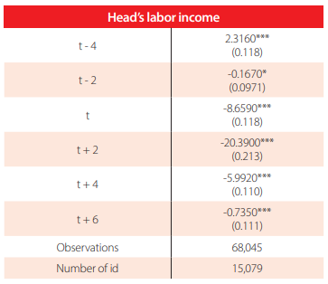
Ordered Logistic Regression Estimates
Notes: Robust standard errors in parentheses.The dependent variable of the regression is the head’s labor income deciles distribution generated by the predicted values based on the estimates of Fixed-effects fourth regression.
*** p < 0.01, ** p < 0.05, * p < 0.1 Source: 1973-2017 PSID waves.
The pre-displacement gap is less significant, which corroborates the hypothesis stated by Gibbons who says that wages before displacement should not differ among groups [11]. Moreover, it is worth noticing that the effect of displacement begins with a relatively small negative shock, and it increases two years after it. The job searching costs or the labor market signal of low productivity due to displacement can explain these annual losses on earnings increases
Table 5 shows the predicted probabilities of being in each decile. Its columns are each income decile, whereas the rows are the time subject to analysis. It displays the calculation of marginal effects for each possible outcome of the ordered logistic regression. The impact of displacement is not significant at 5% four years before displacement. However, two years before displacement and the following periods, every effect is significant at 1% level. Also, no marginal effects are significant in the sixth income decile.
| First Decile (%) | Second Decile (%) | Third Decile (%) | Fourth Decile (%) | Fifth Decile (%) | ||
| t-4 | 0.0473* | 0.0571* | 0.3322* | 0.5034* | 0.8079* | |
| t-2 | -0.6567*** | -0.7942*** | -4.6162*** | -6.9953*** | -11.2257*** | |
| t | 2.4556*** | 2.9694*** | 17.2603*** | 26.1555*** | 41.9731*** | |
| t+2 | 5.7833*** | 6.9934*** | 40.6507*** | 61.6003*** | 98.8534*** | |
| t+4 | 1.6994*** | 2.0550*** | 11.9449*** | 18.1006*** | 29.0471*** | |
| t+6 | 0.2084*** | 0.2520*** | 1.4646*** | 2.2194*** | 3.5615*** | |
| Sixth Decile (%) | Seventh Decile (%) | Eighth Decile (%) | Nineth Decile (%) | Tenth Decile (%) | ||
| t-4 | 0.0170 | -1.5458* | -0.2103* | -0.0088* | -0.0002* | |
| t-2 | -0.2367 | 21.4788*** | 2.9219*** | 0.1220*** | 0.0023*** | |
| t | 0.8849 | -80.3099*** | -10.9250*** | -0.4562*** | -0.0085*** | |
| t+2 | 2.0841 | -189.1425*** | -25.7301*** | -1.0745*** | -0.0201*** | |
| t+4 | 0.6124 | -55.5777*** | -7.5605*** | -0.3157*** | -0.0059*** | |
| t+6 | 0.0751 | -6.8145*** | -0.9270*** | -0.0387*** | -0.0007*** | |
Ordered Logistic Regression Marginal Effects
Notes: Ordered logistic regression marginal effects (dy/dx) using predicted deciles from fixed-effects regression as the dependent variable *** p < 0.01, ** p < 0.05, * p < 0.1Source: 1973-2017 PSID waves
In contrast with the transition matrices results, adding control variables reduces the effects four years before displacement. It means that the differences among groups are not different from zero in this period. Previous productivity similarities between groups can explain these results. It is more likely to be in the seventh decile two years before displacement, showing labor market attachment. Nevertheless, it is more probable that the individual is in the fifth decile in the displacement year and less likely to be in the seventh decile. The results denote the significant impact of being displaced in the moment when it happens. As Jolly explains, the immediate effect of involuntary job losses is the reduction of the labor earnings that are the reward of being involved in the workforce [6].
These adverse effects become more prominent two years after displacement than the year of displacement. The probability of being in the fifth decile is 57 pp. higher than the same point in the year of displacement. Moreover, there is tremendous increase of the probability of being in the fourth and third decile. It shows that being displaced implies a movement of at least two deciles downward the year of displacement and two years after it. The analysis made by Ormiston sheds some light on these results [16]. He explores the role of the worker’s depreciated value following displacement. It can emerge because of foregone returns of specific human capital lost on the previous employer-employee relationship or by a mismatch of the skills set denoting variations in the displaced workers’ potential productivity.
This effect leaves sequels four years after, where it exhibits a negative probability of being in any decile up to the sixth one. Also, it is more likely to be in the fifth decile of predicted annual labor income. These results explain that when the worker can look for other sources of income, either by employment or entrepreneurship, the effect of being displaced begins to vanish. For this reason, there is a deeper decline in the probability of being under the fifth decile. However, the difference of marginal predictions of being on the seventh decile and upward remains negative.
CONCLUSIONS
In this work, I argued that job displacement influences inter-temporal income mobility using annual labor earnings to measure financial well-being. For this, I used the Panel Study of Income Dynamics (1973-2017), the most comprehensive longitudinal data for the US population. This large data set allowed me to observe the income shock persistence due to an involuntary job loss.
My empirical strategy relies on the methodology proposed by [6], which consists of recovering transition matrices probabilities. My main contribution is the use of ordered logistic regression estimators to control for demographic traits that may affect income mobility. This addition allowed me to improve the biases of my estimations with the transition matrices. Moreover, I used clustered standard errors at the unit of analysis level, providing more precise coefficients. Also, by using an extensive period of analysis, I extended the years analyzed before displacement.
I found that displacement triggers a significant reduction of annual labor income, and this effect remained even four years after the job loss occurs. Also, displacement affects income mobility over time, and there were deep earnings losses that increased downward mobility not only when displacement occurred. Downward mobility is deeper two years afterward than in other periods. Displacement’s negative influence on mobility mitigates as time goes by.
One area of improvement is the extension of the financial well-being measure used to study inter-temporal labor income mobility. It can be addressed by considering other measures of well-being like the couple’s labor earnings, family income, wealth, and consumption expenses. Therefore, allowing the analysis of how family members’ income influences income mobility and how wealth and consumption patterns change due to displacement. To conclude, the main findings of this work describe, comprehensively, the inter-temporal persistence of the adverse effects of an involuntary job loss.
AUTHORS' CONTRIBUTIONS
Nicolle Jaramillo had generated all the content embedded in this article
CONFLICTS OF INTEREST
Nicolle Jaramillo declares no conflicts of interest.
REFERENCES
[1] Bruce C Fallick. A review of the recent empirical literature on displaced workers. ILR Review, 50(1):5-16, 1996.
[2] Lori G. Kletzer. Job displacement. Journal of Economic Perspectives, 12(1):115-136, March 1998.
[3] Louis S Jacobson, Robert J LaLonde, and Daniel G Sullivan. Earnings losses of displaced workers. The American economic review, pages 685-709, 1993.
[4] Christopher J Ruhm. Are workers permanently scarred by job displacements? The American economic review, 81(1):319-324, 1991.
[5] Ann Huff Stevens. Persistent effects of job displacement: The importance of multiple job losses. Journal of Labor Economics, 15(1, Part 1):165-188, 1997.
[6] Nicholas Jolly. Job displacement and the inter-temporal movement of workers through the earnings and income distributions. Contemporary Economic Policy, 31(2):392-406, 2013.
[7] Steve Berry, Peter Gottschalk, and Doug Wissoker. An error components model of the impact of plant closing on earnings. The Review of Economics and Statistics, pages 701- 707, 1988.
[8] Maury Gittleman and Mary Joyce. Have family income mobility patterns changed? Demography, 36(3):299-314, 1999.
[9] Kenneth A. Couch and Dana W. Placzek. Earnings losses of displaced workers revisited. American Economic Review, 100(1):572-89, March 2010.
[10] M Lachowska, A Mas, and SA Woodbury. Sources of displaced workers’ long-term earnings losses (working paper no. 24217). National Bureau of Economic Research, 10:w24217, 2018.
[11] Robert Gibbons and Lawrence F Katz. Layoffs and lemons. Journal of labor Economics, 9(4):351-380, 1991.
[12] John T Addison and Pedro Portugal. Job displacement, relative wage changes, and duration of unemployment. Journal of Labor economics, 7(3):281-302, 1989.
[13] David S Kaplan, Gabriel Martinez Gonzalez, Raymond Robertson, Naercio Menezes-Filho, and Omar Arias. What happens to wages after displacement?[with comments]. Economia, 5(2):197-242, 2005.
[14] Daniel Fackler, Steffen Muller, and Jens Stegmaier. Explaining wage losses after job displacement: Employer size and lost firm rents. Technical report, IWH Discussion Papers, 2017.
[15] Ben Kriechel and Gerard A Pfann. Heterogeneity among displaced workers. ROA Maasricht, 2003.
[16] Russell Ormiston. Worker displacement and occupation-specific human capital. Work and Occupations, 41(3):350- 384, 2014.
[17] Thomas A DiPrete. Life course risks, mobility regimes, and mobility consequences: A comparison of sweden, germany, and the united states. American journal ofSociology, 108(2):267-309, 2002.
[18] George A Akerlof. The market for “lemons”: Quality uncertainty and the market mechanism. In Uncertainty in economics, pages 235-251. Elsevier, 1978.
[19] Jacob Mincer. Investment in human capital and personal income distribution. Journal of political economy, 66(4):281-302, 1958.
Notes