

Seasonal-To-Interannual Variability of Sea-Surface Temperatures in the Inter-Americas Seas: PatternDependent Biases in the Regional Ocean Modeling System
Variabilidad estacional e interanual de la temperatura superficial en los mares interamericanos: patrones de sesgo en el sistema regional de modelación del océano
ACI Avances en Ciencias e Ingenierías
Universidad San Francisco de Quito, Ecuador
Recepción: 30 Octubre 2020
Aprobación: 13 Julio 2021
Resumen: Los mares interamericanos (IAS), que se extienden desde el Golfo de México, el Caribe y la parte trópico-oriental del Océano Pacífico que limita con América Central, Colombia y Ecuador; presentan interacciones muy activas entre el océano, el suelo y la atmósfera, que influyen en las actividades socioeconómicas dentro y fuera de la región. Estas interacciones aún no se comprenden en su totalidad y no se representan adecuadamente, inclusive en modelos de última generación. En escalas de tiempo estacionales e interanuales, la principal fuente de variabilidad en esta zona geográfica, se relaciona con las interacciones entre los océanos Pacífico y Atlántico, incluyendo patrones anómalos de la temperatura en la superficie del mar (SST), como El Niño-Oscilación del Sur (ENSO), y otras características regionales relacionadas con la estacionalidad bimodal del chorro de bajo nivel del Caribe. Este estudio investiga las anomalías estacionales e interanuales de los registros de la temperatura en superficie en los mares interamericanos, y de los resultados simulados con una resolución a una escala de remolino, de 1/9° (0.11°, aproximadamente 10 km), generados por el Sistema Regional de Modelado del Océano (ROMS), y en base del Reanálisis del Sistema de Pronóstico del Clima para el período 1999-2008. En lugar de analizar los sesgos de los resultados del modelo de manera local (cuadrícula por cuadrícula), se realizó un diagnóstico no local, en base de la identificación de patrones de la SST, mediante un análisis de componentes principales. Los resultados indican que incluso con resoluciones a escala de remolino, y a diferencia del consenso de la literatura, persisten varios sesgos. El enfoque permitió cuantificar la magnitud, la varianza y los errores sistemáticos de los patrones espaciales de la SST, relacionados con la piscina cálida del hemisferio occidental, ENSO, el Dipolo de los mares interamericanos y otros componentes de variabilidad. Estos sesgos se relacionan principalmente con errores la cuantificación de los flujos de calor en la superficie, una inadecuada representación de las interacciones entre el mar y la atmósfera, componentes que afectan el enfriamiento latente en superficie en la zona del Caribe y genera una estratificación térmica subterránea excesiva, principalmente frente a la costa de Ecuador y el norte de Perú.
Palabras clave: mares interamericanos, Sistema Regional de Modelización del Océano (ROMS), evaluación de modelos en base de patrones.
Abstract: The Inter-Americas Seas (IAS), involving the Gulf of Mexico, the Caribbean and a section of the eastern tropical Pacific Ocean bordering Central America, Colombia and Ecuador, exhibits very active ocean-land-atmosphere interactions that impact socioeconomic activities within and beyond the region, and that are still not well understood or represented in state-of-the-art models. On seasonal-to-interannual timescales, the main source of variability of this geographical area is related to interactions between the Pacific and the Atlantic oceans, involving anomalous sea-surface temperature (SST) patterns like El Nino-Southern Oscillation (ENSO), and regional features in the Caribbean linked to the bi-modal seasonality of the Caribbean Low-Level Jet. This study investigates seasonal-to-interannual IAS surface-temperature anomalies in observations, and their representation in an eddy-permitting, 1/9° or 0.11°; approximately 10 km) resolution simulation using the Regional Ocean Modeling System (ROMS), interannually-forced by the Climate Forecast System Reanalysis for the study period 1999-2008. Here, rather than analyzing model biases locally (i.e., gridbox-by-gridbox), a non-local SST patternbased diagnostic was conducted via a principal component analysis. Regarding spatial resolution, the results of this study suggest that even at eddy-permitting resolutions of 0.11o several biases remain, which contrast with the general consensus in the literature. The approach permitted the identification of magnitude, variance and spatial systematic errors in SST patterns related to the Western Hemisphere Warm Pool, ENSO, the Inter-Americas Seas Dipole, and several other variability modes. These biases are mainly related to errors in surface heat fluxes, misrepresentation of air-sea interactions impacting surface latent cooling in the Caribbean, and too strong sub-surface thermal stratification, mostly off the coast of Ecuador and northern Peru.
Keywords: Inter-Americas Seas, Regional Ocean Modeling System (ROMS), patternbased model evaluation.
INTRODUCTION
Sea-surface temperatures (SST) are key to understanding physical mechanisms regulating regional and global climate at multiple timescales. In the Inter-Americas Seas (IAS), normally referred to as “Intra-Americas Seas,” a region involving the Eastern Tropical Pacific, the Gulf of Mexico and the Caribbean, SST patterns are subject to large spatial and temporal biases in state-of-the-art modeling systems, especially in boreal summer and fall. Several reasons have been suggested for these biases [1-6], including a misrepresentation of the observed area, magnitude and location of the Western Hemisphere and the Atlantic Warm Pool (WHWP and AWP, respectively); model underestimation of latent heat and downwelling shortwave fluxes, but overestimation of sensible heat fluxes in the region; and inadequate representation of interactions between air-sea turbulent fluxes with the low-level easterlies, in turn connected [1-2] to the variability of the North Atlantic Subtropical High (NASH). With significant Global Climate Models (GCMs) biases prevalent in surface fluxes and ocean circulation over the region, it is not surprising to note such large SST model errors over the IAS, and the related misrepresentation of rainfall fields [6].
The availability of quality observational datasets is key to further understanding the physical mechanisms that need to be better represented in the models, and the IAS is one of the most poorly observed regions in the world [7]. Among the first oceanographic studies in the Eastern Tropical Pacific are those of the ASKOY expedition in 1941 [8], involving a cruise that navigated the Panama Bight, integrated by the maritime jurisdictional areas of Panama, Colombia and Ecuador. Years later, in 1965, a description of the oceanographic conditions in this region was conducted, including physical, chemical and biological parameters obtained on board the Colombian Navy’s vessel Bocas de Ceniza, through the Augmented Colombian El Niño-Tuna Oceanographic expedition, ACENTO [9].
By 1976, this type of oceanographic research activities was consolidated within the framework of the Estudio Regional del Fenómeno de El Niño (Regional Study of the El Niño Phenomenon, or ERFEN by its initials in Spanish) as one of the commitments that Colombia acquired as member ofthe Permanent Commission ofthe South Pacific (CPPS). To date, fifty-nine scientific expeditions have been conducted, whose records have allowed to further the knowledge of the oceanic and atmospheric dynamics in the region, which has helped characterize anomalies associated with the occurrence of El Niño-Southern Oscillation (ENSO) events [10]. Frequently unknown to the wider scientific community, these expeditions have produced different technical publications, some of which have been compiled in reports by the Centro de Investigaciones Oceanográficas e Hidrográficas del Pacífico Colombiano (Center for Oceanographic and Hydrographic Research of the Pacific, or CCCP). Another more recent example is the Colombian Atlas of Oceanographic Data [11], which presents climatologies of temperature, salinity and density at different standard depths. Although these investigations have furthered the understanding of oceanographic conditions in the area, the low temporal resolution available due to the small number of oceanographic cruises carried out per year (two at best) limits the full characterization of the dynamics at interannual and seasonal timescales.
One way of palliating the existing regional limitations in the availability of this kind of data is through the use of the numerical ocean models. Although several model simulations exist, few evaluations exist of how well these products represent key oceanic features in this complex region.
Among the numerical models used in the study of ocean circulation processes at regional level, the Regional Ocean Modeling System (ROMS) stands out [12-13]. This model solves the hydrostatic, incomprehensible fluid primitive equations using "terrainfollowing" curvilinear vertical coordinates [14]. ROMS has been used by the Colombian Navy since 2012 following the operational forecast configuration of the Latin American Observatory for Climate Events [15], but this is the first report of the formal evaluation conducted on the model.
The main objective of this study is to identify how well oceanic conditions, specifically sea-surface temperature patterns, are represented in a realistically-forced interannual simulation in ROMS in the IAS. To accomplish this goal, a pattern-based evaluation approach is reported, focusing on the analysis of observed and simulated key modes of SST variability along the year. In the following section the region of study is described. Data and methods are introduced in Section 3, followed by the main results in Section 4. The overall discussion of the results is presented in Section 5, and the concluding remarks are summarized in Section 6.
STUDY AREA: THE INTER-AMERICAS SEAS
The Inter-Americas Seas is part of the WHWP, defined as a broad area including the Gulf of Mexico, southern United States, Mexico, the Caribbean Sea with its islands, Central America, northern South America, and the ocean off the west coast of Central America and Colombia (Fig. 1).
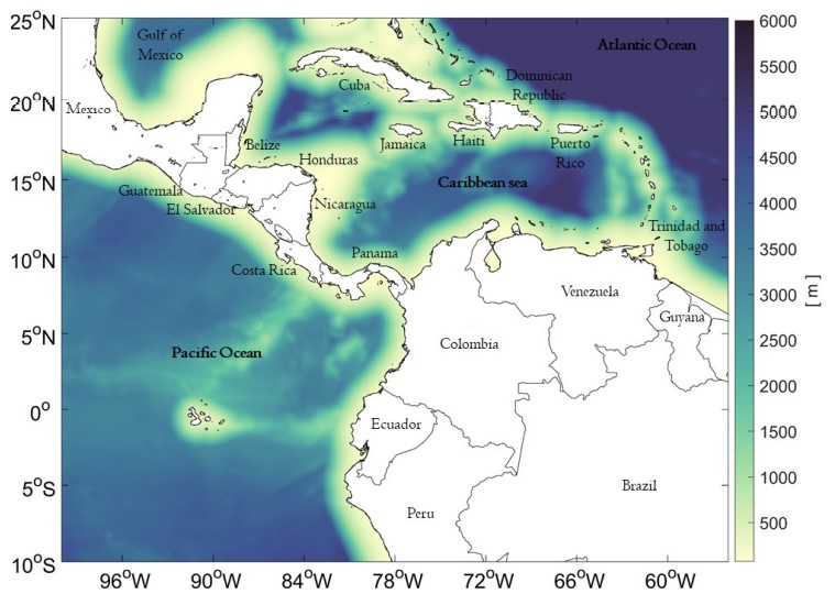
Geographical area of study in the Inter-Americas Seas. Colors represent depth in meters below mean sea level.
According to some authors, the WHWP is related to the genesis of the warm and cold phases of ENSO [16-17]. Between the boreal summer and autumn, the WHWP exhibits a peak in SST [18-19] that dominates most of the eastern tropical Pacific region [20-21], crossing Central America to encompass areas of the Caribbean and the Central Atlantic Ocean.
During winter (December to February, DJF), the Inter-Tropical Convergence Zone (ITCZ) is at its most southern position, and the northeastern trade winds intensify in the region [22]. The difference in atmospheric pressure between the Gulf of Mexico and the Caribbean, as well as in the Tropical Pacific Ocean (TPO), is related to the presence of the Caribbean Low-Level Jet (CLLJ, [23-24]) and the bi-annual incursion of NASH in the region of interest [25], with intense winds that cross the mountainous area of Central America and interact with other low-level jets in the gulfs of Tehuantepec, Papagayo and Panama [26-27]. The Papagayo Jet crosses the depression of Lake Nicaragua and rises on the Pacific coast, about 70 km north of the Gulf of Papagayo, near San Juan del Sur, Nicaragua. The Panama Jet extends from the coastal area of the Gulf of Panama, centered around 79°W, to the Ecuadorian maritime territory. As a result of the interaction of these jets with the upper ocean layer, there is a coastal upwelling (Ekman positive pumping) that generates a zonal gradient in the SST in the Panama Bight region, as well as in the maritime territory of Mexico and Nicaragua in the Pacific Ocean [23-24, 28]. In general, the SST isotherms over the Caribbean and the eastern tropical Pacific are mostly zonally distributed.
DATA AND METHODS
Interannual simulation using the Regional Ocean Modeling System (ROMS)
In the present simulation, the lateral boundary conditions used were taken from the Simple Ocean Data Assimilation (SODA) dataset [29]. The surface forcing of the model was carried out with data from the National Center for Environmental Prediction - Climate Forecast System Reanalysis (NCEP-CFSR), which provides global atmospheric conditions from 1979 to 2010 [30]. These data have a spatial resolution of approximately 38 km (T382), with global coverage and 64 pressure levels.
The Extended Reconstructed Sea-Surface Temperature dataset version 5 (ERSSTv5) provides sea-surface temperature fields at 2 degrees and monthly resolutions for the entire planet, from January 1854 to present [31].
ROMS is a high-resolution model that uses curvilinear coordinates that follow the bathymetry and solves the primitive equations in a rotating reference system (the Earth), based on the Boussinesq approximation and considering hydrostatic [32]. In this study, version 3.0 of ROMS AGRIF was adopted, with which an interannual experiment was carried out through a 12-year period. This model has been implemented previously for the studies in the Southeast Pacific, analyzing the mean circulation, the seasonal cycle, and the mesoscale dynamics of the Peru Current System (PCS; [13]), exhibiting a good representation of the predominant ocean features in this sector. Nonetheless, a pattern-based evaluation of the representation by ROMS of SST patterns in the IAS region has not been conducted until now.
Model configuration
In the implementation of the model, a computational mesh was configured that frames a section of the IAS included in the region defined by 100°W to 56°W, and 10°S to 25°S. The bathymetric information has a resolution of two (2) arc-minutes and was obtained from the global ETOPO2 dataset, which uses observations of depth sounding and satellite altimetry [33].
Although ROMS has terrain-following coordinates that allow for a more realistic representation of the bathymetry, a smoothing of the terrain slopes is used to avoid errors in the pressure gradient [34]. This smoothing is controlled in the model via the rtarget parameter [35], which, after some sensitivity experiments, was assigned a value of 0.15.
The resolution of the simulation is 1/9° (or 0.11°; approximately 10 km) for the construction of the horizontal grid, and 32 levels of depth for the vertical sigma coordinate. For the distribution of the vertical layers, values of surface stretching and bottom stretching, respectively, θS = 6 and θB = 0 were used, corresponding, respectively, to the coordinate parameters for the surface and bottom levels.
A total of 12 years were simulated, from January 1997 to December 2008. By the end of the second simulated year, the volume-averaged kinetic energy reached an asymptotic value. Hence, the first two years were discarded due to the model’s spin-up period, and the remaining 1999-2008 period was used in the analysis. Two simulation years have also been reported by previous studies (e.g., [36, 13]) as a typical time for model stabilization.
Data processing and analysis
The mean seasonal cycle was first subtracted from the sea-surface temperature fields for each non-concurrent season of interest in the period 1999-2008: DJF, MAM, JJA and SON (respectively periods of every three months, December to February, March to May, June to August and September to November). Then a Principal Component Analysis (PCA) was conducted on the sea-surface temperature anomalies, SSTa, for each season using the International Research Institute for Climate and Society’s Climate Predictability Tool (CPTv16; [37]), which computes the Empirical Orthogonal Functions via a singular-value decomposition. The first three Empirical Orthogonal Functions (EOFs) were used for the analysis, typically explaining 73-90% of the total observed variance, depending on the season.
Since the sample size for the PCA is relatively short, a comparison was conducted between the observed EOFs obtained when using the same 10-year period of the simulation (1999-2008), and a 20-year (1994-2014) and a 30-year (1984-2014) period, which included strong El Niño and La Niña events. No major differences were obtained (not shown) in the observed patterns or the explained variance associated with each EOF in any of the seasons, and hence the selected 10-year period was considered enough for the analysis.
Because the spatial horizontal resolution of the simulation does not match the horizontal resolution of the ERSSTv5 dataset, the latter was interpolated from ~0.11° to 2°. Nonetheless, to avoid losing spatial features when computing the PCA, the analysis was also conducted using the original model resolution.
Spatial patterns in the simulation (with and without interpolation) were compared against the observed EOFs for each season, and whenever major differences arose, model biases were related to concrete physical modes of variability and misrepresentation of physical mechanisms in the region.
SEASONAL AND INTERANNUAL VARIABILITY OF SEA-SURFACE TEMPERATURE ANOMALIES IN THE IAS
This section presents the main results of the pattern-based diagnostic analysis, in conjunction with the identification of biases in ROMS based on an extensive literature review for discussion.
DJF season
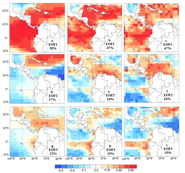
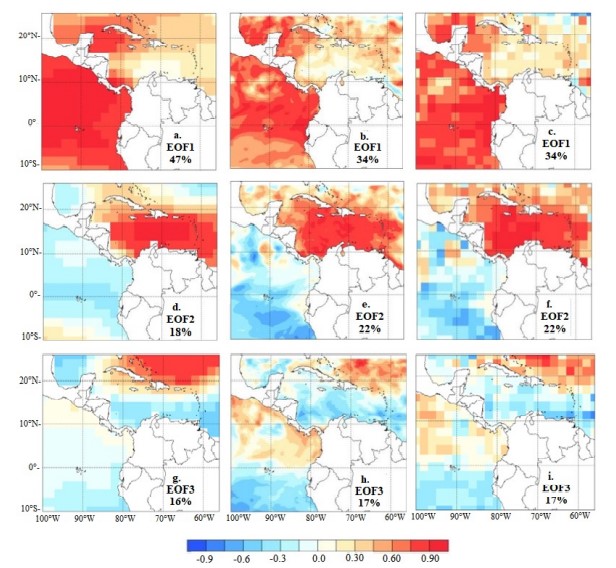
Spatial distribution of the first three modes (rows) of SSTa variability for the DJF season for ERSSTv5 (a, d and g), ROMS (b, e and h) and ROMS interpolated at a resolution of 2° (c, f and i). Each panel displays the explained variance associated with each EOF.
The SSTa spatial pattern identified via the first Empirical Orthogonal Function (EOF1; Fig. 2a) sketches the seasonal imprint of the WHWP covering most of the analysis domain, consistent with the so-called Meridional-Wind Mode [38]. The EOF1 is related to northerly wind anomalies linked to below-normal SST in the Caribbean, and at the same time southeasterly wind anomalies over the Gulf of Mexico, coupled with above normal SST there (Figs. 2a-c). This pattern is also associated with frequency variations of the high-latitude cold air-mass intrusion [39-40]. In this season, ROMS largely captures the main spatial features of the observed pattern (Fig. 2b, c), although the explained variance exhibited by the simulated pattern is ~11% less than the observed one.
The EOF2 (Fig. 2d) exhibits a meridional dipolar structure in the Caribbean region, known as the IAS Dipole, that is mostly driven by changes in the air-sea heat fluxes [17]. A weak structure appears mainly in the maritime zone of Ecuador in the observed EOF2, contrasting with the rest of the eastern Pacific. Contrary to the performance exhibited by ROMS on reproducing the main features of the WHWP seasonal pattern (EOF1), the model erroneously interchanges EOF2 and EOF3 (see middle and bottom rows in Fig. 2), assigning slightly more (~4%) explained variance than it should to the third observed EOF. Furthermore, the simulated EOF3 (cfr. Fig. 2d, h-i) shows biases both in the magnitudes and geographical extension of the IAS Dipole, confining it to the northeastern sector of the domain, showing just a weak signal over and to the west of Cuba.
In addition, ROMS overdoes the observed SSTa pattern over the equatorial Pacific (cfr. Fig. 2d, h-i), suggesting a warm bias related to a misrepresentation of the weak sub-surface thermal stratification (“thermostad”) observed in the region [41] and reported in certain ROMS configurations [42]. The higher spatial resolution of ROMS allows resolving the effects on SSTa of the Tehuantepec, Papagayo and Panama Low-Level Jets in the Pacific Ocean region in the observed EOF2, an influence that is also observed in EOF3, especially in the case of the Panama Jet. Nonetheless, their impact on SST fields cannot be formally evaluated in this work, as ERSSTv5 does not resolve them adequately. This topic deserves further analysis and will be discussed in a future study.
The Caribbean section of the observed EOF3 (Fig. 2g) is related to the seasonal intensification of the CLLJ, bringing cooler-than-average SSTa off the coast of northern South America (Fig. 2e, f), in part contributing to rainfall inhibition during this season. Except for the fact that ROMS confused EOF2 and EOF3, the magnitudes and spatial patterns are represented by the model, although the SSTa pattern off the coast of Ecuador is stronger than it should be, suggesting again model biases related to subsurface thermal stratification.
The actual difference in the explained variance of the simulated EOF2 and EOF3 is ~1% (cfr. Fig. 2e, h), explaining the inversion in the ordering of the simulated EOFs. Nonetheless, the same difference in the ERSSTv5 dataset is ~5% (Fig. 2d, g). Even when these differences can be considered small, they are important when analyzing the modes of variability that most contribute to explain the SSTa variance and indicate biases in the physical processes represented in the model.
MAM season
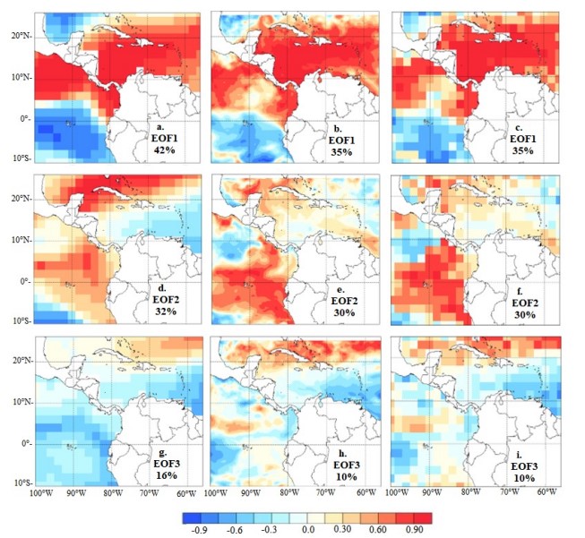
Spatial distribution of the first three modes (rows) of SSTa variability for the MAM season for ERSSTv5 (a, d and g), ROMS (b, e and h) and ROMS interpolated at a resolution of 2° (c, f and i). Each panel displays the explained variance associated with each EOF.
In this season, the first observed spatial pattern explaining most of the SSTa variance (EOF1, Fig. 3a) is consistent with the WHWP SST distribution in both the Pacific and the Caribbean. Although ROMS assigns a lower explained variance (~7% less than the observed one; cfr. Fig. 3a-c) to this mode of variability, it tends to reproduce the large- scale features observed, related to a homogeneous pattern of SST between 27°C and 28°C present in the Caribbean Sea during the season [43].
EOF2 (Fig. 3d) shows a spatial distribution associated with an IAS [17, 38], which is characterized by late-winter and early-spring positive SSTa in the Caribbean Sea and negative SSTa in the Gulf of Mexico. This dipole pattern is not really present in the ROMS simulation (Fig. 3e-f), suggesting biases related to the representation of surface heat fluxes over the Caribbean and the Gulf of Mexico. Nonetheless, the simulation assigns to this mode a value of the explained variance that is similar to the one observed (a difference of ~2%). This relatively high explained variance in the simulation is related to the model assigning a large statistical charge to the spatial pattern in the eastern tropical Pacific, related to ENSO, which otherwise exhibits a similar spatial distribution to the ERSSTv5 (Fig. 2d-f).
The observed EOF3 (Fig. 3g) corresponds to the “Transition Mode” [38], exhibiting a dipolar pattern in the Caribbean but contrasting with the IAS Dipole (EOF2) because the signal is almost absent in the Gulf of Mexico, and does not extend into the Pacific, which shows a mostly homogeneous spatial distribution of SST. Compared to the observed EOF3, ROMS exhibits in the Pacific a zonally-distributed SSTs pattern of opposite sign along 5°N and also a noisy SSTa region off the coast of Ecuador and northern Peru; similarly, the simulation shows a dipolar structure too strong and extending farther west into the Gulf of Mexico, compared to the observed pattern (Fig. 3h, i). Furthermore, ROMS underestimates the explained variance for this mode of variability in ~6%.
In summary, in the boreal spring ROMS tends to represent well the spatial features of the ENSO peak season in the Pacific, and the WHWP in the IAS, but there are important biases regarding the representation of the IAS Dipole.
JJA season
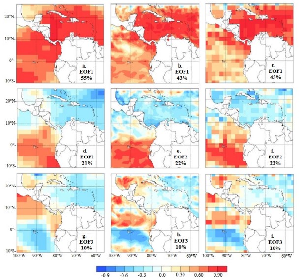
Spatial distribution of the first three modes (rows) of SSTa variability for the JJA season for ERSSTv5 (a, d and g), ROMS (b, e and h) and ROMS interpolated at a resolution of 2° (c, f and i). Each panel displays the explained variance associated with each EOF.
During the JJA season, the WHWP (EOF1; Fig. 4a) pattern has expanded, covering a larger extension than in the previous season in both the Caribbean and the Pacific [18, 4445]. The WHWP normally transitions into the AWP in June and shows a peak typically in early September [1]. This spatial pattern is better represented by ROMS (Fig. 4b, c) in the Caribbean than in the Pacific. Although similar patterns appear in both ERSSTv5 and ROMS off the Pacific coast of Central America, in ROMS the pattern is noisier than the one observed for the rest of the Pacific region (Fig. 4b, c). The difference in explained variance between the observed and simulated EOF1 is ~12%.
Most of the signal in the observed and simulated EOF2 (Fig. 4d-f) appears in the Pacific region, which exhibits a pattern associated with ENSO-like SSTa [46-48]. The simulation and observed explained variances for this mode are basically the same (difference of ~1%), indicating ROMS tends to reproduce adequately the mechanisms related to the spatial distribution of SSTa variability during the mature season of ENSO.
The EOF3 (Fig. 4g-i) resembles the signature of the so-called eastern Pacific SST Cooling Mode [49], with its narrow zonal SSTa pattern extending off the coast of Ecuador and northern Peru. This mode, which ROMS reproduces with the same explained variance as in ERSSTv5 and with a slightly more equatorially confined pattern—probably due to the higher resolution of the simulation—is reported to be related to global warming [49] via a strengthening ofthe zonal SST gradient in the region, enhancing the trade winds, promoting stronger upwelling and thus creating a positive feedback that reinforces the SST contrast. A homogeneous SSTa pattern is observed in both the observed and simulated EOF3 for most of the Caribbean, with an opposite signal in the Gulf of Mexico.
In summary, in the boreal summer the model has a fair representation of the large-scale spatial features of the modes analyzed, and the total explained variances the EOF2 and EOF3, except for the considerably less homogenous signal of the WHWP in the Pacific in EOF1, which consistently exhibits less variance in ROMS than in ERSSTv5.
SON season
Spatial distribution of the first three modes (rows) of SSTa variability for the SON season for ERSSTv5 (a, d and g), ROMS (b, e and h) and ROMS interpolated at a resolution of 2° (c, f and i). Each panel displays the explained variance associated with each EOF.
As with the other seasons, most of the observed explained variance (~47%) is associated with the WHWP (EOF1, Fig. 5a), which exhibits very low SSTa variability in the Caribbean off the coast of Venezuela and Colombia during the SON season [18], and during November involves the AWP demise phase [1]. Although ROMS does capture most of the spatial features (Fig. 5b-c), especially after interpolating at 2o, it assigns an explained variance which is ~13% lower than the observed one.
The second EOF (Fig. 5d-f) corresponds to the Interocean Mode [38, 1] and is related to southwesterly winds that contribute to the formation of the inter-basin dipolar configuration. The pattern also has a contribution related to the second annual weakening of the CLLJ, which favors an increase in positive SSTa [24] between ~12°N-17°N and 80°W- 70°W. The Interocean Mode tends to be enhanced during ENSO events, which modulate the strength of the CLLJ, reinforcing the SSTa dipolar configuration [38, 50]. The main observed spatial feature of the SON EOF2 in the tropical Pacific region resembles an ENSO-type configuration, consistent with previous studies (e.g. [51]). ROMS captures the main spatial features of the inter-basin dipole, but the explained variance is ~4% higher than that of the observed EOF2. Part of this extra variance can be related to the fact that ROMS tends to represent high-resolution features, like the Papagayo Jet (southwest off the coast of Nicaragua), which are less notorious in the ERSSTv5 dataset (Fig. 5d-f). Other differences are related to a local pattern off the coast of Ecuador in the simulation, that is not really visible in ERSSTv5; and a mostly inverted signal, and noisier north of 20°N than the observed pattern, in the Caribbean (Fig. 5d-f).
The Caribbean part of the EOF3, both in ERSSTv5 and ROMS (Fig. 5g-i), resembles the IAS Dipole discussed in the analysis for the DJF season (section 4.1). EOF3 is considered here a precursor of the IAS Dipole, related to the so-called Meridional-Wind Mode [38]. Although the difference in explained variance between the ERSSTv5 and ROMS in this EOF is ~1%, the simulation tends to amplify both in magnitude and areal extension the observed SSTa configuration along the Pacific coast of Central America.
In summary, in the boreal fall the main model spatial-pattern biases are related to a noisy SSTa field north of 20oN (EOF2), and a too strong and too wide SSTa signal in the Pacific, north of the Equator and south of the Central American coast (EOF3).
Main patterns and biases in ROMS
The most common approach when evaluating model biases is to report a variety of statistical metrics to quantify the differences between model output and ERSSTv5. Although this approach is deemed very useful by the scientific community, a drawback is that it tends to lack a direct physical interpretation of the reported errors. For example, frequently used metrics like Pearson’s correlation or Root Mean Square Error can be very useful to quantify how in-phase two variables are, or an average measure of how different the magnitudes of those variables are, respectively, but in and of themselves these metrics do not provide information about which physical processes are not being well represented in the model universe.
Furthermore, the most common approach evaluates biases on a gridbox-by-gridbox (or local) basis, thus making it difficult to assess if particular observed spatio-temporal patterns are being represented in the model. These patterns can in general be shifted, rotated, deformed, rescaled or actually not represented at all in the model world [52].
An alternative approach, used in this study, focuses on the evaluation of the model representation of the most important observed modes of variability of the field of interest—SST in this case—and that helps identify problems in the representation of key physical processes. In brief, a pattern-based evaluation approach permits understanding when the model reproduces the right processes for the right reasons and adds value for both scientific and operational purposes.
Using a Principal Component Analysis to conduct the model pattern-based evaluation has the additional advantage of being able to use a Principal Component Regression (PCR) and other EOF-based methods (see [53]) as bias-correction approaches, also known as calibration or Model Output Statistics [54]. To make the case, consider PCR:
 (1)
(1)Equation (1) builds a linear regression model for the value Yi of the variable of interest (SST in this case), for each gridbox i, where m counts for the maximum number of the model patterns--EOFxj-considered (e.g., m=3 in this study), aij is the slope regression coefficient for the gridbox i and--EOFxj--, and is the corresponding intercept value. In other words, a PCR is a multiple linear regression which uses the model EOFs as predictors rather than each gridbox’s value of the variable under consideration.
Hence, analyzing how well the observed patterns are reproduced by a model also helps to better understand how much of the total bias is associated with each pattern, assessed, for example, via the explained variance reported by each EOF. This is the approach followed in this study, and the EOF analysis and associated variances were described in the previous section.
The simulated patterns do not need to be perfect to be able to conduct a bias-correction through these EOF-based methods. If the most important observed modes of variability are simulated, even with biases that shift their location or rotate them, these methods are in principle able to extract useful information from the model. The Model Output Statistics approach is especially useful when interested in prediction (for an example considering the IAS, see [6]). Although this study does not directly deal with calibration and prediction, these topics underscore the importance of the analysis conducted here regarding better understanding of model biases in the main patterns of variability in ROMS, at least for SSTa in the IAS region.
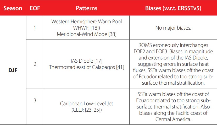
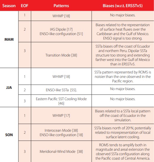
Overall, the main biases are summarized in Table 1. ROMS tends to correctly reproduce the main mode of variability (EOF1) in IAS, characterized by the WHWP signature, in all seasons but the boreal summer. Coincidentally, the second and third modes of variability tend to exhibit different errors in different seasons, but these tend to be less pronounced in the boreal summer. As indicated in the Introduction, most state-of-the- art global models tend to show their largest biases in boreal summer and fall [1-5].
Main patterns and biases in ROMS
Generally speaking, ENSO-like and Pacific SSTa configurations—although sometimes too strong—tend to be better represented than some patterns in the Caribbean and Gulf of Mexico, with some key biases in the IAS Dipole between boreal winter and spring, and SSTa patterns off the coast of Ecuador and northern Peru (winter), and alongshore the Pacific coast of Central America (fall and winter). Consistent with previous studies [1], these errors are suggested here to be related to biases in surface heat fluxes, misrepresentation of the impact of westerly anomalies on surface latent cooling in regions of the Caribbean, and warm biases related to too strong sub-surface thermal stratification. Is it also possible that a component of the biases is related to the assimilation of initial and boundary conditions, as reported by some authors (e.g., [42]).
Regarding spatial resolution, the results of this study suggest that even at eddypermitting resolutions of 0.11° several biases remain, which contrast with the general consensus in the literature [1, 55-56]. It is also true that some spatial features cannot be adequately evaluated using ERSSTv5 due to the relatively low-resolution of the dataset, such as the effects of the Tehuantepec, Papagayo and Panama low-level jets in the Pacific Ocean region. This is another reason why a process-based model evaluation approach is an important complement, as more traditional bias assessment between model and ERSSTv5 when the horizontal resolution is very different can be misleading, even after interpolation to a common horizontal resolution.
CONCLUDING REMARKS
This study investigated variance and spatial biases in sea-surface temperature patterns in the Inter-Americas Seas, represented by a 0.11° resolution, interannually-forced simulation using the Regional Ocean Modeling System. Rather than using a variety of statistical metrics to assess local (i.e., gridbox-by-gridbox) differences between the simulation and data based on observations (ERSSTv5), the study focused on analyzing if the sea-surface temperature patterns that explain most of the total observed variance are present in the simulation, and, if so, which are the main biases exhibited by each pattern. Furthermore, the study analyzed the most likely physical processes involved in those pattern-dependent biases.
The large-scale spatial features and variances related to the Western Hemisphere Warm Pool and ENSO-like patterns tend to be well represented in the model in most but not all seasons. Overall, spatial biases are more frequently present in the Caribbean and Gulf of Mexico than in the eastern Pacific region under study, with magnitude, variance and areal extension biases related to the Inter-Americas Seas Dipole (boreal winter and spring), and the Transition (spring), Interocean and Meridional-Wind (fall) modes. The analysis suggests that model biases are mainly related to errors in surface heat fluxes, misrepresentation of air-sea interactions impacting surface latent cooling in the Caribbean, and too strong sub-surface thermal stratification, typically off the coast of Ecuador and northern Peru.
The fact that several pattern-dependent biases exist in the eddy-permitting, relatively high-resolution simulation conducted suggests that important errors remain even in configurations running at high horizontal resolution and that additional work is needed to improve model representation of physical processes and adequate assimilation of initial and boundary conditions.
ACKNOWLEDGEMENTS
This study is part of ALCL’s PhD thesis work at Jorge Tadeo Lozano University (Colombia). ÁGM and XC were partially supported by the NOAA Award NA18OAR4310275.
DECLARATIONS FUNDING
The Climate Predictability Tool software is available here: https://iri.columbia.edu/cpt
AUTHORS' CONTRIBUTIONS
ALCL and AGM designed the study, analyzed the results and drafted the manuscript. ALCL conducted and analyzed the model simulations. XC and SL provided support for running the model and post-processing its output. All co-authors reviewed and approved the manuscript.
Referencias
Misra, V. (2020) Regionalizing Global Climate Variations: A Study of the Southeastern US Regional Climate. Elsevier Science. https://doi.org/10.1016/6-0-04147-7
Misra, V., & Chan, S. (2009) Seasonal predictability of the Atlantic Warm Pool in the NCEP CFS. Geophysics Research Letter 36: L16708. https://doi.org/10.1029/2009GL039762
Kozar, M., & Misra, V. (2013) Evaluation of twentieth-century Atlantic Warm Pool simulations in historical CMIP5 runs. Climate Dynamics 41:2375-2391. https://doi:10.1007/s00382-012-1604-9
Liu, Y., Lee, S.K., Muhling, B.A., Lamkin, J.T., & Enfield, D.B. (2012) Significant reduction of the Loop Current in the 21st century and its impact on the Gulf of Mexico. Journal of Geophysical Research 117C05039. https://doi:10.1029/2011JC007555
Ryu, J.H., & Hayhoe, K. (2014). Understanding the sources of Caribbean precipitation biases in CMIP3 and CMIP5 simulations. Clim Dyn 42, 3233-3252. https://doi.org/10.1007/s00382-013-1801-1
Krishnamurthy, L., Muñoz, A., Vecchi, G., Msadek, R., Wittenberg, B., & Gudgel, F. (2018) Assessment of summer rainfall forecast skill in the Intra-Americas in GFDL high and low-resolution models. Climate Dynamics 52:1965-1982. https://doi.org/10.1007/s00382-018-4234-z
IASCLIP (2005). A prospectus for an Intra-Americas Study of Climate Processes (IASCLIP). Report prepared by the VAMOS panel. https://doi:10.1029/2002JD002089
Wooster, W.S. (1959) Oceanographic Observations in the Panamá Bight, ''ASKOY" expedition, 1941. New York: Bulletin of the American Museum of Natural History. Volume 118:117-151.
Forsbergh, E. (1969) Sobre la Climatología, Oceanografía y Pesquerías del Panamá Bight, IATTC, 14 (2).
Caicedo, A. L., Muñoz, C. C., Iriarte, J. D., Gutiérrez, M. A., Rojas, E. J., & Quintero, K. D. (2020). Capitulo III - Aproximación a la variabilidad estacional e interanual de las condiciones oceanográficas en la Cuenca Pacífica Colombiana. En Compilación Oceanográfica de la Cuenca Pacífica Colombiana II. (Pp. 100-133). Dirección General Marítima. Bogotá, D. C. Editorial Dimar.
Andrade, C., Rangel, O., Herrera, E. (2015). Atlas de los Datos Oceanográficos de Colombia 1922-2013 Temperatura, Salinidad, Densidad, Velocidad. Dirección General Marítima-Ecopetrol S.A. Ed. Dimar. Bogotá, Colombia. https://doi.org/10.26640/9789585897809.2015
Melsom, A., Lien, V., & Budgell., W. (2009) Using the Regional Ocean Modeling System (ROMS) to improve the ocean circulation from a GCM 20th century simulation. Ocean Dynamics. https://doi.org/10.1007/s10236-009-0222-5
Penven, P., Echevin, V., Pasapera, J., Colas, F., & Tam, J. (2005) Average circulation, seasonal cycle, and mesoscale dynamics of the Peru Current System: A modeling approach. Journal Geophysical Research. https://doi.org/10.1029/2005JC002945
Penven, P., Cambon, G., & Tan, T. (2010) ROMS AGRIF / ROMSTOOLS. User Guide. Institut de Recherche pour le Developpement (IRD)
Muñoz, A.G., López, P., Velásquez, R., Monterrey, L., León, G., Ruiz, F., Recalde, C., Cadena, J., Mejía, R., Paredes, M., Bazo, J., Reyes, C., Carrasco, G., Castellón, Y., Villarroel, C., Quintana, J., & Urdaneta, A. (2010b). An Environmental Watch System for the Andean Countries: El Observatorio Andino. Bulletin of the American Meteorological Society 91(12): 1645-1652. https://doi.org/10.1175/2010BAMS2958.1
Park, J., Kug, J., Li, T., & Behera, S.K. (2018). Predicting El Niño Beyond 1-year Lead: Effect of the Western Hemisphere Warm Pool. Scientific Reports. https://doi.org/10.1038/s41598-018-33191-7
Muñoz, E., Wang, C., & Enfield, D. (2010). The Intra-Americas Springtime Sea Surface Temperature Anomaly Dipole as Fingerprint of Remote Influences. Journal of Climate. https://doi.org/10.1175/2009JCLI3006.1
Wang C, Enfiel, DB (2001) The Tropical Western Hemisphere Warm Pool. Geophysical Research Letters. https://doi:10.1029/2000GL011763
Wang, C., Fiedler, P. (2006). ENSO variability in the eastern tropical Pacific: A review. Progress in Oceanography 69:239266. https://doi.org/10.1016/j.pocean.2006.03.004
Da Silva, A.M., Young, C., & Levitus, S. (1994) Atlas of Surface Marine Data 1994, vol. 1, Algorithms and Procedures. NOAA Atlas NESDIS 6, US Department of Commerce, NOAA, NESDIS, USA, 74pp
Magaña, V., Amador, J.A., & Medina, S. (1999). The midsummer drought over Mexico and Central America. Journal Climate 12:1577-1588. http://dx.doi.org/10.1175/15200442(1999)012<1577:TMD0MA>2.0.C0;2
Srinivasan, J., & Smith, G. (1996). Meridional migration of tropical convergence zones. Journal of Applied Meteorology 35:1189-1202. https://doi.org/10.1175/1520-0450(1996)035<1189:MMOTCZ>2.0.CO;2
Amador, J.A., Alfaro, E.J., Lizano, O.G., & Magaña, V.O. (2006). Atmospheric forcing of the eastern tropical Pacific: A review. Progress in Oceanography 69: 101-142. https://doi.org/10.1016/j.pocean.2006.03.007
Amador, J.A. (2008). The Intra-Americas sea low level jet: overview and future research. Ann N Y Acad Sci 1146:153-88. https://doi:10.1196/annals.1446.012
Wang, C. (2007). Variability of the Caribbean Low-Level Jet and its relations to climate. Climate Dynamics 29:411-422. https://doi.org/10.1007%2Fs00382-007-0243-z
Chelton, D.B., Freilich, M.H., & Esbensen, S.K. (2000). Satellite observations of the wind jets off the Pacific coast of Central America. Part I: Case studies and statistical characteristics. Monthly Weather Review. https://doi. org/10.1175/1520-0493(2000)128<1993:SOOTWJ>2.0.CO;2
Chelton, D.B., Esbensen, S.K., Schlax, M.G., Thum, N., & Freilich, M.H., Wentzb, F.J., Gentemannb, C.L., McPhaden, M.J., & Schopf, P.S. (2001). Observations of Coupling between Surface Wind Stress and Sea Surface Temperature in the Eastern Tropical Pacific. Journal of Climate 14(7):1479-1498. https://doi.org/10.1175/1520-0442(2001)014<1479:OOCBSW>2.0.CO;2.
Lizano, O.G. (2016). Distribución espacio-temporal de la temperatura, salinidad y oxígeno disuelto alrededor del Domo Térmico de Costa Rica. Revista de Biología Tropical. https://doi:10.15517/rbt.v64i1.23422
Carton, J., Giese, B., & Grodsky, S. (2005). Sea level rise and the warming of the oceans in the Simple Ocean Data Assimilation (SODA) ocean reanalysis. Journal of Geophysical Research 110:C09006. https://doi:10.1029/2004JC002817
Saha, S., Shrinivas, M., Pan, H., Wu, X., Wang, J., Nadiga, S., Tripp, P., Kistler, R., Woollen, J., Behringer, D., Liu, H., Stokes, D., Grumbine, R., Gayno, G., Wang, J., Hou, Y., Chuang, H.,Juang, H., Sela, J., Iredell, M., Treadon, R., Kleist, D., Delst, P., Keyser, D., Derber, J., Michael, E., Meng, J., Wei, H., Yang, R., Lord, S., Dool, H., Kumar, A., Wang, W., Long, C., Chelliah, M., Xue, Y., Huang, B., Schemm, J., Ebisuzaki, W., Lin, R, Xie, P., Chen, M., Zhou, S., Higgins, W., Zou, C., Liu, Q., Chen, Y., Han, Y., Cucurull, L., Reynolds, R.W., Rutledge, G., & Goldberg, M. (2010). The NCEP Climate Forecast System Reanalysis. Bulletin of the American Meteorological Society 91(8):1015-1057. https://doi.org/10.1175/2010BAMS3001.1
Huang, B., Thorne, P.W., Banzon, V.F., Boyer, T., Chepurin, G., Lawrimore, J.H., Menne, M.J., Smith, T.M., Vose, R.S., & Zhang, H.M. (2017). Extended Reconstructed Sea Surface Temperature version 5 (ERSSTv5), Upgrades, validations, and intercomparisons. J. Climate, doi: https://doi.org/10.1175/JCLI-D-16-0836.1
Shchepetkin, A.F., & McWilliams, J.C. (2005). The regional oceanic modeling system (ROMS): A split-explicit, free- surface, topography-following-coordinate oceanic model. Ocean Modelling 9:347-404. https://doi.org/10.1016/j.ocemod.2004.08.002
Smith, W., & Sandwell, D. (1997). Global seafloor topography from satellite altimetry and ship depth soundings. Science 277:1956-1962. https://doi:10.1126/science.277.5334.1956
Haney, R. (1991). On the pressure force over steep topography in sigma coordinate ocean models. Journal of Physical Oceanography 21: 610-619. https://doi.org/10.1175/1520-0485(1991)021<0610:OTPGFO>2.0.CO;2
Beckmann, A., & Haidvogel, D.B. (1993). Numerical simulation of flow around a tall isolated seamount, Part I, Problem formulation and model accuracy. Journal of Physical Oceanography 23:1736-1753. https://doi.org/10.1175/1520- 0485(1993)023<1736:NSOFAA>2.0.CO;2
Marchesiello, P., McWilliams, J.C., & Shchepetkin, A. (2003). Equilibrium Structure and Dynamics of the California Current System. Journal Physical Oceanography. https://doi.org/10.1175/1520-0485(2003)33<753:ESADOT>2.0.CO;2
Mason, S., Tippet, M., Song, L., & Muñoz, A.G. (2020). Climate Predictability Tool version 16.5.2. Columbia University Academic Commons. https://doi.org/10.7916/d8-z7qf-4z45.
Rodriguez, G., Romero, R., Castro, C., & Castro, V. (2019). Coupled Interannual Variability of Wind and Sea Surface Temperature in the Caribbean Sea and the Gulf of Mexico. Journal of Climate 32:4263-4279. https://doi.org/10.1175/JCLI-D-18-0573.1.
Legeckis, R. (1988). Upwelling off the Gulfs of Panama and Papagayo in the tropical Pacific during March 1985. Journal of Geophysical Research. https://doi.org/10.1029/jc093ic12p15485
Zárate, E. (2013). Climatología de masas invernales de aire frío que alcanzan Centroamérica y el Caribe y su relación con algunos índices Árticos. Tópicos Meteorológicos y Oceanográficos 12:35-55.
Kessler, W. (2006). The circulation of the eastern tropical Pacific: A review, Prog. Oceanogr., 69, 181-217, doi: https://doi.org/10.1016/j.pocean.2006.03.009
Echevin, V., Colas, F., Chaigneau, A., & Penven, P. (2011). Sensitivity of the Northern Humboldt Current System nearshore modeled circulation to initial and boundary conditions, Journal of Geophysical Research: Oceans. Blackwell Publishing Ltd, 116(7), p. C07002. doi: https://doi.org/10.1029/2010JC006684
Martínez, C., Goddard, L., Kushnir, Y., & Ting, M. (2019). Seasonal climatology and dynamical mechanisms of rainfall in the Caribbean 53: 825-846. Climate Dynamics. https://doi.org/10.1007/s00382-019-04616-4.
Misra, V., Li, H., Kozar, M. (2014). The precursors in the Intra Americas seas to seasonal climate variations over North America. Journal Geophysical Research (Oceans) 119(5): 2938-2948. https://doi.org/10.1002/2014JC009911
Cruz, D.C. (2018). Estructura Dinámica y Termodinámica del Calentamiento Atmosférico en la Climatología de Colombia. Disertación. Universidad Nacional de Colombia.
L’Heureux, M.L., Collins, D.C., & Hu, Z.Z. (2013). Linear trends in sea surface temperature of the tropical Pacific Ocean and implications for the El Niño-Southern Oscillation. Climate Dynamics 40:1223-1236. https://doi:10.1007/s00382-012-1331-2.
Hoerling, M.P., & Kumar, A. (2003) The perfect ocean for drought. Science 299: 691-694. https://doi.org/10.1126/science.1079053
Rodgers, K.B., Friederichs, P., & Latif, M. (2004). Tropical Pacific decadal variability and its relation to decadal modulation of ENSO. Journal Climate 17:3761-3774. https://doi.org/10.1175/1520-0442(2004)017<3761:TPDVAI>2.0.CO;2
Zhang, W., Li, J., Zhao, X. (2010). Sea surface temperature cooling mode in the Pacific cold tongue. Journal of Geophysical Research 115:C12042. https://doi.org/10.1029/2010JC.
Serna, L., Arias, P., & Vieira, S. (2018). The Choco and Caribbean low-level jets during El Niño and El Modoki events. Revista de la Academia Colombiana de Ciencias Exactas, Físicas y Naturales. http://dx.doi.org/10.18257/raccefyn.705
Deser, C., Alexander, M., Xie, S., & Phillips, A. (2010). Sea Surface Temperature Variability: Patterns and Mechanisms 2:115-145. Annual Review of Marine Science. https://doi.org/10.1146/annurev-marine-120408-151453
Muñoz, A.G., Yang, X., Vecchi, G., Robertson, A., & Cooke, W. (2017). A Weather-type based Cross-Timescale Diagnostic Framework for Coupled Circulation Models. Journal of Climate 30:8951-8972. https://doi.org/10.1175/JCLI-D-17-0115.1
Tippett, M., DelSole, T., Mason, S., & Barnston, A. (2008). Regression-based methods for finding coupled patterns. Journal of Climate 21(17):4384-4398. https://doi.org/10.1175/2008JCLI2150.1
Wilks, D. S., (2006). Statistical Methods in the Atmospheric Sciences. 2nd ed. Elsevier, 627 pp.
Misra, V., & Mishra, A. (2016). The oceanic influence on the rainy season of Peninsular Florida. Journal Geophysical Research:Atmosphere 121:7691-7709. https://doi.org/10.1002/2016JD024824
Chérubin, L.M., Sturges, W., & Chassignet, E.P. (2005). Deep flow variability in the vicinity of the Yucatan Straits from a high-resolution MICOM simulation. Journal Geophysical Research. https://doi.org/10.1029/2004JC002280