

Simple Hardware Implementation of Motion Estimation Algorithms
Implementación simple en hardware de algoritmos para la estimación de movimiento
ACI Avances en Ciencias e Ingenierías
Universidad San Francisco de Quito, Ecuador
Received: 15 January 2019
Accepted: 17 June 2019
Abstract: In the following work is presented a hardware implementation of the two principal optical flow methods. The work is based on the methods developed by Lucas & Kanade and Horn & Schunck. The implementation is made by using a field programmable gate array and Hardware Description Language. To achieve a successful implementation, the original algorithms were optimized. The results show the optical flow as a vector field over one frame, which enables an easy detection of the movement. The results are compared to a software implementation to ensure the success of the method. The results are a fast implementation capable of quickly overcoming a traditional implementation in software.
Keywords: Horn & Schunck, Lucas & Kanade, FPGA, VHDL, Movement, Derivative, Optical Flow.
Resumen: En el siguiente trabajo se presenta la implementación en hardware de los dos métodos principales de flujo óptico. El trabajo se basa en los métodos desarrollados por Lucas & Kanade y Horn & Schunck. La implementación se realiza mediante una matriz de puertas lógicas programables en campo y en lenguaje de descripción de hardware. Para lograr una exitosa implementación los algoritmos originales fueron optimizados. Los resultados muestran el flujo óptico como un campo vectorial sobre un cuadro del video, lo que permite una fácil detección del movimiento. Los resultados se comparan con una implementación de software para asegurar el éxito de los métodos. Los resultados son una implementación veloz capaz de superar en rapidez a una implementación tradicional en software.’
Palabras clave: Horn & Schunck, Lucas & Kanade, FPGA, VHDL, Movimiento, Derivada, Flujo Óptico.
INTRODUCTION
Computer vision intends to understand, in a mathematical way, the biological process of the interaction eye-brain with the tridimensional world, and to capture this stimulus in a systematic model compatible with an electronic device (for signal processing) [1-3]. Progress in technology has enabled the development of hardware and software letting a machine simulate comprehension, to a certain level, of some physical phenomena. Development in the field of computer science has enabled the optimization of algorithms, therefore machines get information and interact with the real world in a more efficient way [1-3].
Vision can turn on a complex subject when a model is interpreted in a mathematical way. The human brain uses the information that comes from the eyes and processes it. When the information is processed, the brain makes some assumptions to interpret parameters such as depth, brightness reflection over a surface, and the relative movement of an object [1-3]. All these assumptions enable us to construct a 3D model of the environment. When these processes are simulated by a computer, they become a great challenge because they are based on complex physical, mathematical and even statistical models [1-6].
Movement of objects in the real world induces a change in the 2D plane inside images [1-3]. This change can be described as a variation in the brightness patterns and can be analyzed between two frames of a video [3]. Optical flow describes the distribution of the apparent velocities of these changes of patterns [4-6]. In case of absence of change on the light from the source, the change of position brightness pattern between two or more images can be detected as movement [1-2]. This is a comprehensive concept if it is considering the definition of movement on video as well as the edge detection and if certain restrictions are considered as explained later. Optical flow is the pattern created by the relative movement of an object between two images, typically between two frames of a video. The optical flow result is a vector field where the movement is presented with vectors (arrows) [1-3]. While the movement is greater, so the vectors will be.
There are some motion estimation algorithms implemented in hardware, but most of them havea complex implementation [7-8]. The objective of this work is to present an innovative and simple way to implement the calculi of optical flow in hardware.To do so, the two principal and classical optical flow algorithms are tested. These algorithms are Lucas & Kanade and Horn & Schunck [4-5]. The reason these two algorithms are chosen is that they are classical algorithms that have proved to be reliable [6]. To implement the algorithm, a Field programmable gate array (FPGA) is chosen, mainly because of the relative low computing time. The algorithms are implemented in the FPGA in a hardware description language (HDL). The novelty of this work lies on a fast implementation of the optical flux algorithms over an FPGA.
METHODS
Edge Detection and Estimation of Derivatives by Finite Differences
Abrupt changes of brightness in an image can be useful data for image processing. Algorithms that detect these changes are known as edge detection algorithms [8-10]. The borders of objects generate abrupt changes of luminosity when compared with the image’s background. [1,3]. One of these abrupt changes (border) is described as a considerable gradient of the brightness in one or more segments of the image [1].To calculate the gradient of brightness inside a digital image, it is necessary to approximate the derivatives, using the finite differences, as Eq. 1 shows [1,3].
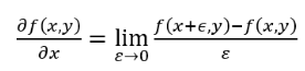 (1)
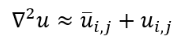
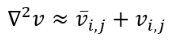
(1)It is also mandatory to know the laplacian operator when trying to solve a problem of optimization, as proposed by Horn & Schunck [4] and Lucas & Kanade [5] for optical flow calculation. Eq. 2 shows the laplacian operator [1-3].
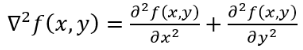 (2)
(2)ALGORITHMS
Assumptions
To compute an optical flow, two assumptions are needed. The first one is called Brightness Constancy assumption. It is assumed the brightness stays constant between two consecutive frames of a video, as Eq. 3 [4-6,9-10] shows, where E represents the brightness in the position x, y, t.
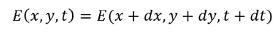 (3)
(3)From the idea generated in Eq. 3, it is reasonable to assume that the partial derivatives of E will be zero. Eq. 4 describes the brightness constancy assumption, where Ex, Ey and Et are the space and time partial derivatives of the frame [6,8-11]. The values . and . are the horizontal and vertical components of a vector that show how a pixel moves from frame one to frame two. This vector is called optical flow when calculated for every pixel in the image.
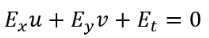 (4)
(4)The second one is called Smoothness Constraint assumption. The smoothness constraint suggests that all pixels conforming an object of finite dimensions inside an image (brightness pattern) tend to move as a rigid body, so it is unusual to find pixels moving independently to their neighbors [6,8-11]. Therefore, the velocity field will vary smoothly in almost every part of the image. The smoothness constraint implies the minimization of the space partial derivatives of the velocity components. It is accomplished using the Eq. 5 and 6, where and represent the local averages of the velocity components [6,8-11].
 (5)
(5)
 (6)
(6)Lucas & Kanade
The algorithm presented by Lucas & Kanade segments the image in neighborhoods (square windows) for the calculation of partial optical flow. After optical flow is calculated for each neighborhood, it will be generalized for the entire neighborhood [5-6,8-10,12]. The method developed by Lucas & Kanade applies both the brightness constancy assumption and the smooth constancy to solve the optical flow equation by optimizing an energy functional. Eq. 7 represents the matrix model given by this method, where the derivative sub-indexes represent the number of the pixel being analyzed. This matrix model can be solved obtaining the optical flow components for the velocity of movement. In other words, Eq. 7 is the generalization of Eq. 4 and when solved the components of all velocity vectors are found. Every pixel will have one associate velocity vector representing how much that pixel is moving from frame to frame.
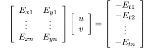 (7)
(7)Horn & Schunck
The method developed by Horn & Schunck uses the brightness constancy assumption and the smoothness constraint to solve the optical flow equation. This method suggests the minimization of two errors given by the constraints used, as shown in Eq. 8 and 9, where εb is the brightness constancy error and εc is the smoothness error [4,6,8-11]:
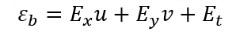 (8)
(8)
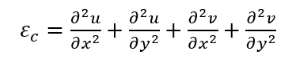 (9)
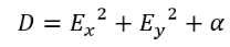
(9)With help of variation calculus, finite differences and Eq. 4-5, 8-9 the derivatives to minimize the error are computed. Eq. 10-13 show a numerical solution for u and v [4,6,8-11]. is a fixed parameter, normally a natural number less than 10.
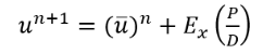 (10)
(10)
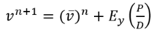 (11)
(11)In Eq. 10 and 11, n represents the number of iterations. For iteration ni the calculus will be done for the entire matrix. Using that result the algorithm will proceed to do the calculus for the iteration ni+1.
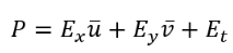 (12)
(12)
 (13)
(13)HARDWARE IMPLEMENTATION
To implement the algorithm, the software Vivado from Xilinx is used. The code in every module in HDL uses a synchronous programming. In other words, every action is executed at each clock rising edge. The synchronous coding is very important because otherwise there would be issues synchronizing the modules. Moreover, each module begins when a flag is raised, and when the module is done, it notifies another flag. Using this idea each module needs an enabled flag to start and generate an ending flag, allowing the modules to start only when they should.
Flux Diagram
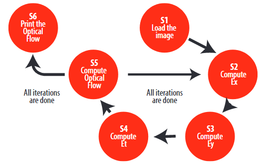
The implementation follows a process that involves several steps as shown in Figure 1. In this process, the coordinates of each vector are calculated by two different methods (Horn & Schunck algorithm and Lucas & Kanade algorithm). Each pixel in the image will have a vector associated with it. The vector will show the motion of the pixel between the two frames.
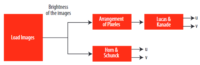
Flux Diagram
Module Description
Loading the Image
The two starting images are grayscale; in other words, they are monochromatic images. The images are coded in 8 Bits in binary. This encryption allows having 256 possible values of color between black and white. The values of the color are handled as integer where zero is black and two hundred fifty-five is white. To load the images, the pixel´s values of brightness are written in a text file. Then these values are copied in our first module. The values are set in two vectors that contain values of brightness.
The vector size is the same as the number of pixels in the image. To sum up, the load Image module is in fact a ROM memory handwritten. This ROM memory contains the two Images to be processed.
Arrangement of pixels
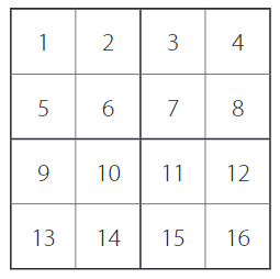
Rearrangement of Pixels into small square window
In Lucas & Kanade algorithm, images are divided into little square windows of either two or four pixels. The last option is shown in Fig 2. The aim of this module is to facilitate the calculation of the Lucas & Kanade algorithm. Indeed, the input vector contains the values of the pixels by increasing the position. When calculating the coordinates of the vector, the values will be grouped by window. It is therefore desirable to rearrange the vector as follows:
[1,2,3,4,5,6,7,8....16]
becomes [1,2,5,6,3,4,7,8...16]
With this rearrangement, the useful values for each calculation are side by side in the vector. This reorganization depends on the window size chosen. The reorganization should be done to all the windows that conform the image.
Lucas & Kanade
The module implements Eq. 7. To do this, the partial derivatives of space and time are computed, and then the values of u and v. In order to implement this, Eq. 7 is split into small calculations. This small calculation is the spatial and time derivate. Finally, the module assembly all calculi together. In other words, the module solves the matrix equation in the form of several tensor equations. In digital images all the values of the position (x, y, t) of the pixels are natural numbers. Fig. 3 shows the details of the module solving Eq. 7. Fig. 3 shows the Finite State Machine (FSM) used to implement this module.
FSM to implement Lucas and Kanade Module
Horn & Schunck
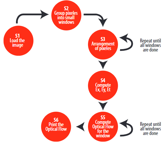
The module implements the Eq. 10 and 11. With that, the values u and v of each vector are computed. Only the result obtained after the number of desired iterations is displayed. The module needs the number of iterations. The decision of how many iterations are needed could be challenging. Several iterations too small result in a miscalculation, and an overextended number of iteration results in a too high computing time. The images in the results section were obtained using 50 as the iteration number. In the discussion section will be more information about this number. Fig. 4 shows in detail how the module implements the numerical solution for Eq. 10 and 11 using a Finite State Machine (FSM).
State Machine to Implement Horn & Schunck Module
RESULTS
Fig. 5 shows the two frames to test the algorithms implemented. Fig. 5a is the first frame and 5b is the second frame of a video. The main movement is in the trunk of the car. In addition, there is a slight movement at the level of the man. Next important results consist of evaluating the optical flow result for each method (Lucas & Kanade and Horn & Schunck). Each arrow represents the motion of each pixel between the first and the second image. In Horn & Schunck´s algorithm, the number of iterations is critical; a higher number of interactions produces better results but generates a higher time in the synthesis step during the HDL compilation. The time elapsed in the synthesis step is closely related to the processor and memory of the computer where it is done. The number of iterations that best fit our resources were around 50. The price to obtain better results is a higher synthesis time.
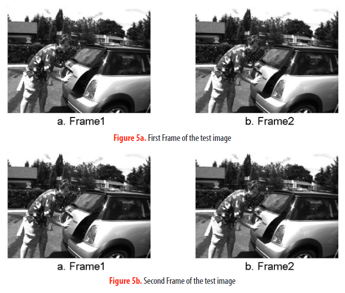
Original Images to test
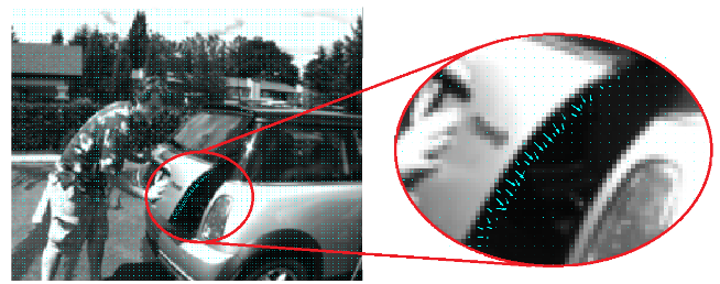
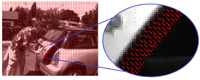
Optical Flow computed using Lucas & Kanade’s algorithm in VHDL
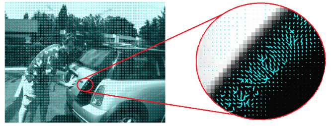
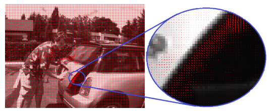
Optical Flow computed using Horn & Schunck’s algorithm in VHDL
Optical Flow computed using Lucas & Kanade’s algorithm in MATLAB
computed using Horn & Schunck’s algorithm in MATLAB
| Platform | Algorithm | Time |
| Matlab | Lucas & Kanade | 172 us |
| Horn & Schunck | 195 us | |
| HDL | Lucas & Kanade | 50 ns |
| Horn & Schunck | 51 ns |
Average Time Comparison
Table 1 registers how much time it takes to compute the components of the velocity vector for each pixel inside the image. It is important to remark that Table 1 shows the required time to compute the velocity vector for one pixel inside the image. To obtain the total time, this number should be multiplied by the total number of pixels in the image. Moreover, it is important to remember that it is an average time.
DISCUSSION
The specificity of the two algorithms is evaluated and compared based on two parameters: strengths and limits. In order to compare our FPGA’s implementation, we implement the algorithms in a traditional way in MATLAB as shown in Figs. 8 and 9. MATLAB’s implementation has better precision due to the difficulty in carrying the decimal in FPGA’s implementation. The decimal difficulty arises because the values of intensity (of the image) are handled in integer format. The solution for the decimals problem is to multiply the brightness values by one hundred before the calculi and afterward do a shift by two to the left. The shift by two means the decimal is pushed two positions to the left, similar to an arithmetic division by one hundred. The solution presented to the decimals problem tries to preserve two decimal precision. The implementation in VHDL is quite faster than MATLAB because it is implemented in hardware inside the FPGA.
Figs.6-7 show the hardware implementation. Figs.8-9 show the MATLAB’s implementation. Comparing Figs 6-7 with 8-9, it is noticeable that MATLAB’s implementation images have more arrow density that VHDL images. The lower arrow density is because the used FPGA has a limited memory, and therefore it is imperative to load images with low resolution. Table 1 shows a time comparison between the time elapsed to compute the velocity vector for each pixel in the image. The time is computed for each pixel instead of for each image. The images have different resolutions, so comparing the time per image would not be appropriate.
Both algorithms have some limitations; for example, rotation movements are not well detected. In that case, the algorithms will detect the movement, but not all the arrows will be in the right direction. The problem exists because the frames of a video are a 2D representation of a 3D world. In addition, both algorithms (Lucas & Kanade and Horn & Schunck) have the same goal: to show the motion of each pixel between the first and the second image. However, small differences can be observed in the results. In the case of the Lucas & Kanade algorithm, there is a strong detection of the main movement, but small movements (notably at the level of the man in Fig. 5) are not easily detected. For Horn & Schunck, small movements are well detected, but the direction of the strongest movement is less trustful, in comparison with Lucas & Kanade. Moreover, the computation time for Horn & Schunck is higher, as shown in Table 1, because the algorithm needs a greater number of iterations. This effect can be seen in both implementations: MATLAB and VHDL, as it is noticeable in Table 1. It is then suggested by the results of Figs. 6-9 that Lucas & Kanade has better quality results and, according to Table 1, is the fastest one; therefore, it is more suitable for a real time application.
Two motion estimations algorithms have been successfully implemented in hardware: Lucas & Kanade and Horn & Schunck. They are implemented on FPGA by using VHDL language, and their results are compared with software implementation. The results obtained clearly show the movement, but each algorithm and implementation has its own differences. The algorithm is very reliable to detect 2D movement, but when the movement includes rotation, the direction detected is not always the right one. The innovative VHDL implementation is faster than a conventional software implementation (MATLAB) due to the fact that it is a hardware implementation. Finally, in a timing analysis, Lucas & Kanade’s algorithm is the best option to implement a real time application.
REFERENCES
[1] Horn, B. K., & Schunck, B. G. (1981). Determining optical flow. Artificial intelligence, 17(1-3), 185-203. doi: https://doi.org/10.1016/0004-3702(81)90024-2
[2] Lucas, B. D., & Kanade, T. (1981). An iterative image registration technique with an application to stereo vision.
[3] Bruhn, A., Weickert, J., & Schnörr, C. (2005). Lucas/Kanade meets Horn/Schunck: Combining local and global optic flow methods. International journal of computer vision, 61(3), 211-231. doi: https://doi.org/10.1023/B:VISI.0000045324.43199.43
[4] Mallot, H. A. (2000). Computational vision: information processing in perception and visual behaviour. MIT Press.
[5] Pratt, W. K. (2007). Digital Image Processing: PIKS Scientific inside. Wiley-Interscience, John Wiley & Sons, Inc.
[6] Harris, D., & Harris, S. (2010). Digital design and computer architecture. Morgan Kaufmann.
[7] Kruger,W., Enkelmann, W., & Rossle, S. (1995, September). Real-time estimation and tracking of optical flow vectors for obstacle detection. In Proceedings of the Intelligent Vehicles’ 95. Symposium (pp. 304-309). IEEE.
[8] Zach, C., Pock, T., & Bischof, H. (2007, September). A duality based approach for realtime TV-L 1 optical flow. In Joint pattern recognition symposium (pp. 214-223). Springer, Berlin, Heidelberg.
[9] Honegger, D., Meier, L., Tanskanen, P., & Pollefeys, M. (2013, May). An open source and open hardware embedded metric optical flow cmos camera for indoor and outdoor applications. In 2013 IEEE International Conference on Robotics and Automation (pp. 1736-1741). IEEE.
[10] Barron, J. L., Fleet, D. J., Beauchemin, S. S., & Burkitt, T. A. (1992, June). Performance of optical flow techniques. In
[11] Brox, T., Bregler, C., & Malik, J. (2009, June). Large displacement optical flow. In 2009 IEEE Conference on Computer
[12] Stanisavljevic, V., Kalafatic, Z., & Ribaric, S. (2000). Optical flow estimation over extended image sequence. In 2000