

Sección C: Ingenierías
Potential of neural networks for structural damage localization
Potencial de redes neuronales para localización de daño estructural
ACI Avances en Ciencias e Ingenierías
Universidad San Francisco de Quito, Ecuador
ISSN: 1390-5384
ISSN-e: 2528-7788
Periodicity: Bianual
vol. 11, no. 2, 2018
Received: 15 November 2018
Accepted: 17 December 2018
Corresponding author: abambres@netcabo.pt

Abstract: Fabrication technology and structural engineering states-of-art have led to a growing use of slender structures, making them more susceptible to static and dynamic actions that may lead to some sort of damage. In this context, regular inspections and evaluations are necessary to detect and predict structural damage and establish maintenance actions able to guarantee structural safety and durability with minimal cost. However, these procedures are traditionally quite time- consuming and costly, and techniques allowing a more effective damage detection are necessary. This paper assesses the potential of Artificial Neural Network (ANN) models in the prediction of damage localization in structural members, as function of their dynamic properties – the three first natural frequencies are used. Based on 64 numerical examples from damaged (mostly) and undamaged steel channel beams, an ANN-based analytical model is proposed as a highly accurate and efficient damage localization estimator. The proposed model yielded maximum errors of 0.2 and 0.7 % concerning 64 numerical and 3 experimental data points, respectively. Due to the high- quality of results, authors’ next step is the application of similar approaches to entire structures, based on much larger datasets.
Keywords: Structural Health Monitoring, Damage Localization, Steel Beams, Dynamic Properties, Natural Frequencies, Artificial Neural Networks.
Resumen: Los avances de la tecnologia de fabricacion y de la ingenieria estructural han conducido a la utilización crescente de estructuras esbeltas, y consecuentemente mas vulnerables a acciones estáticas y dinámicas que puedan generar algun tipo de daño. En este contexto, inspecciones regulares y evaluaciones son necesarias para detectar y predecir daño en las estructuras, y estabelecer acciones de mantenimiento que puedan garantizar la seguridad y durabilidad estructurales bajo un costo optimizado. Sin embargo, estos procedimientos son tipicamente muy morosos y costosos, y tecnicas que permitan una deteccion del daño de forma mas efectiva son necesarias. Este articulo evalua el potencial de las redes neuronales artificiales (ANN, en Inglés) en la prediccion de la localización del daño en elementos estructurales, como funcion de las caractaeristicas dinámicas de los mismos – las trés primeras frequencias naturales de vibracion son utilizadas. Basado en 64 ejemplos numericos de vigas en acero con seccion en ‘canal’, con (mayoritariamente) y sin daño, este trabajo propone un modelo analitico basado en ANN que es caracterizado por una alta precision y eficiencia. El modelo propuesto originó errores de 0.2 y 0.7% relativamente a 64 y 3 puntos experimentales, respectivamente. Debida a la elevada calidad de los resultados, el proximo paso de estes autores sera la aplicación de abordagenes similares a estructuras completas de puentes o edificios, consecuentemente involucrando bases de datos mucho más volumosas.
Palabras clave: Monitoreo de salud estructural, Localización de daño, Vigas en Acero, Propiedades Dinámicas, Frecuencias Naturales, Redes Neuronales Artificiales.
Introducción
Fabrication technology and structural engineering states-of-art have led to a growing use of slender structures in construction industry. Those structures (or structural members) are more susceptible to static and dynamic actions that may lead to damage and/or excessive vibration. In this context, regular inspections and evaluations are necessary to detect and predict structural damage and establish maintenance actions able to guarantee structural safety and durability with minimal cost. However, these procedures are traditionally quite time-consuming and costly. Thus, techniques allowing a more efficient and less resource-dependent damage detection are in high demand and will contribute to a more sustainable built environment.
In recent years, several authors (e.g., [1-3]) have concluded that structural damage detection is a problem of pattern recognition, in which a classification is made as function of physical properties of a system. Within machine learning, several types of Artificial Neural Networks (ANN) (e.g. feedforward nets, self-organizing maps, learning vector quantization) can become a quite effective damage detection tool when used in conjunction with the dynamic properties of a system (e.g., [4-5]) – note that nowadays is quite straight forward the accurate estimation of important dynamic properties (e.g., natural frequencies) of (possibly damaged) built structural systems (by means of accelerometers and/or other simple decices, and existing software – e.g., ARTeMIS Modal 4.0 [6]). According to Bandara et al. [7] and Ahmed [8], a clear challenge concerning ANNs is the fact that they typically need structural data of both damaged and intact structures to be able to classify satisfactorily. If the structure is not considered damaged in its current state, the information regarding the damaged state will be unavailable unless detailed structural models are used to generate this information, such as numerical ones based on the Finite Element Method (FEM).
Several authors have published the application of machine learning for damage characterization in structural members (e.g., [9-12]). Nonetheless, none of those studies employed exactly the same structure and input/output variables considered in this work. Moreover, the accuracy provided by those solutions are typically insufficient (maximum error for all data points > 5%) for what the authors of this paper consider to be acceptable (safe) in structural engineering practice. Thus, this paper primarily aims to assess the potential of ANN-based models in the prediction of damage localization in structural members, as function of their dynamic properties – the three first natural frequencies are used in this work. Based on numerical data from damaged (mostly) and undamaged steel channel beams, an ANN-based analytical model is proposed and tested for both numerical and experimental data. Once proved that the approach taken works well for structural members, authors’ next step (in the very near future) is to apply similar procedures to entire bridge or building structures.
DATA GATHERING
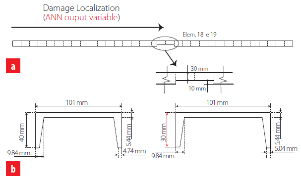
Inspired by the experimental research of Brasiliano [13], who assessed the effect of structural damage on natural (free vibration) frequency values, the data used for the present investigation concerns damaged (mostly) and undamaged ASTM A36 steel channel beams (U101.6x4.67 [14]) with a length of 2.155 m and free-free boundary conditions. Sixty-four distinct beams (also called examples or data points in this manuscript) were simulated in ANSYS FEA software [15] to obtain a 3-input and 1-output dataset for ANN design. The three first natural frequencies (Hz) of the beam are the input (independent) variables – see Tab. 1, whereas the damage location is the output (dependent) variable. The latter is given by the longitudinal distance (m) from beam’s edge to the mid-point of local cross-section reduction that defines the damage (see Fig. 1(a)). For the 13 undamaged beams, the damage location adopted is non- null, randomly taken below 0.005 m, an approach typically providing better ANN-based approximations, according to authors’ experience.
| Vibration Mode | Undamaged Beam | Damaged Beam | ||||
| Test (Hz) | FEA (Hz) | Error FEA vs Test (%) | Test (Hz) | FEA (Hz) | Error FEA vs Test (%) | |
| 43.66 | 42.54 | 2.6 | 39.59 | 41.14 | 3.9 | |
| 120.11 | 117.04 | 2.6 | 117.31 | 117.19 | 0.1 | |
| 235.01 | 229.00 | 2.6 | 222.88 | 222.22 | 0.3 | |
Timoshenko beam FEs of type BEAM188 [15], characterized by six degrees of freedom per node, were employed in all numerical models. For validation purposes, the first two models were used to predict the three first natural frequencies of two beams tested by Brasiliano [13] (also reported in [16]). These beams are characterized by the material and geometrical properties mentioned before, being one undamaged/intact and the other not. The latter was divided into 33 equal longitudinal elements and a 10 mm reduction of its cross-section (shortening of both flanges) was performed in elements 18 and 19, as illustrated in Fig. 1. Tab. 1 presents the validation results in terms of natural frequencies, as well as the corresponding numerical modal shapes. The maximum error of 3.9 % indicates the suitability of the FE model for the present study. Once validated the numerical model, 50 other damage scenarios were simulated, varying damage extent and/or location. The last 12 models were made without damage but under different temperatures from -5 to 40 degrees Celsius. Considering a room temperature of 22 °C, distinct Young moduli were adopted as proposed by Callister and Rethwish [17]. The dataset used in ANN design can be found online in [18]. Next section provides all details concerning the ANN formulation, analyses and results.
ARTIFICIAL NEURAL NETWORKS
Introduction
Machine learning, one of the six disciplines of Artificial Intelligence (AI) without which the task of having machines acting humanly could not be accomplished, allows us to “teach” computers how to perform tasks by providing examples of how they should be done [19]. When there is abundant data (also called examples or patterns) explaining a certain phenomenon, but its theory richness is poor, machine learning can be a perfect tool. The world is quietly being reshaped by machine learning, being the Artificial Neural Network (also referred in this manuscript as ANN or neural net) its (i) oldest [20] and (ii) most powerful [21] technique. ANNs also lead the number of practical applications, virtually covering any field of knowledge [22-23]. In its most general form, an ANN is a mathematical model designed to perform a particular task, based in the way the human brain processes information, i.e. with the help of its processing units (the neurons). ANNs have been employed to perform several types of real-world basic tasks. Concerning functional approximation, ANN-based solutions are frequently more accurate than those provided by traditional approaches, such as multi-variate nonlinear regression, besides not requiring a good knowledge of the function shape being modelled [24].
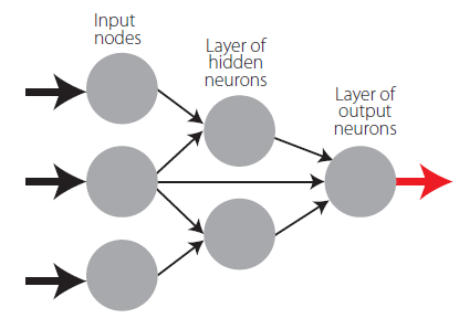
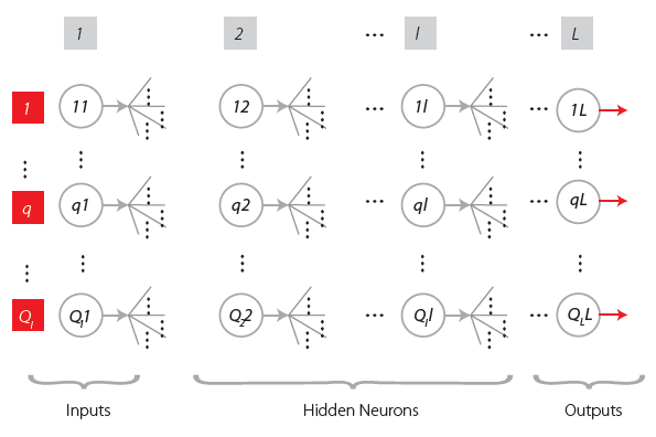
The general ANN structure consists of several nodes disposed in . vertical layers (input layer, hidden layers, and output layer) and connected between them, as depicted in Fig.2. Associated to each node in layers 2 to ., also called neuron, is a linear or nonlinear transfer (also called activation) function, which receives the so-called net input and transmits an output (see Fig. 5). All ANNs implemented in this work are called feedforward, since data presented in the input layer flows in the forward direction only, i.e. every node only connects to nodes belonging to layers located at the right-hand-side of its layer, as shown in Fig. 2. ANN’s computing power makes them suitable to efficiently solve small to large-scale complex problems, which can be attributed to their massively parallel distributed structure and (ii) ability to learn and generalize, i.e, produce reasonably accurate outputs for inputs not used during the learning (also called training) phase.
Learning
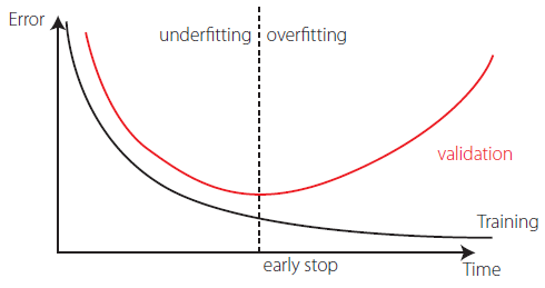
Each connection between 2 nodes is associated to a synaptic weight (real value), which, together with each neuron’s bias (also a real value), are the most common types of neural net unknown parameters that will be determined through learning. Learning is nothing else than determining network unknown parameters through some algorithm in order to minimize network’s performance measure, typically a function of the difference between predicted and target (desired) outputs. When ANN learning has an iterative nature, it consists of three phases: (i) training, (ii) validation, and (iii) testing. From previous knowledge, examples or data points are selected to train the neural net, grouped in the so-called training dataset. Those examples are said to be “labelled” or “unlabeled”, whether they consist of inputs paired with their targets, or just of the inputs themselves – learning is called supervised (e.g., functional approximation, classification) or unsupervised (e.g., clustering), whether data used is labelled or unlabeled, respectively. During an iterative learning, while the training dataset is used to tune network unknowns, a process of cross-validation takes place by using a set of data completely distinct from the training counterpart (the validation dataset), so that the generalization performance of the network can be attested. Once “optimum” network parameters are determined, typically associated to a minimum of the validation performance curve (called early stop – see Fig. 3), many authors still perform a final assessment of model’s accuracy, by presenting to it a third fully distinct dataset called “testing”. Heuristics suggests that early stopping avoids overfitting, i.e. the loss of ANN’s generalization ability. One of the causes of overfitting might be learning too many input-target examples suffering from data noise, since the network might learn some of its features, which do not belong to the underlying function being modelled [25].
Implemented ANN features
The “behavior” of any ANN depends on many “features”, having been implemented 15 ANN features in this work (including data pre/post processing ones). For those features, it is important to bear in mind that no ANN guarantees good approximations via extrapolation (either in functional approximation or classification problems), i.e. the implemented ANNs should not be applied outside the input variable ranges used for network training. Since there are no objective rules dictating which method per feature guarantees the best network performance for a specific problem, an extensive parametric analysis (composed of nine parametric sub-analyses) was carried out to find‘the optimum’net design. A description of all implemented methods, selected from state of art literature on ANNs (including both traditional and promising modern techniques), is presented next – Tabs. 2-4 show all features and methods per feature. The whole work was coded in MATLAB [26], making use of its neural network toolbox when dealing with popular learning algorithms (1-3 in Tab. 4). Each parametric sub-analysis (SA) consists of running all feasible combinations (also called “combos”) of pre-selected methods for each ANN feature, in order to get performance results for each designed net, thus allowing the selection of the best ANN according to a certain criterion. The best network in each parametric SA is the one exhibiting the smallest average relative error (called performance) for all learning data. It is worth highlighting that, in this manuscript, whenever a vector is added to a matrix, it means the former is to be added to all columns of the latter (valid in MATLAB).
Qualitative Variable Representation (feature 1)
A qualitative variable taking . distinct “values” (usually called classes) can be represented in any of the following formats: one variable taking . equally spaced values in ]0,1], or 1-of-. encoding (boolean vectors – e.g., .=3: [1 0 0] represents class 1, [0 1 0] represents class 2, and [0 0 1] represents class 3). After transformation, qualitative variables are placed at the end of the corresponding (input or output) dataset, in the same original order.
| F1 | F2 | F3 | F4 | F5 | |
| FEATURE METHOD | Qualitative Var Represent | Dimensional Analysis | Input Dimensionality Reduction | % Train- Valid- Test | Input Normalization |
| 1 | Boolean Vectors | Yes | Linear Correlation | 80-10-10 | Linear Max Abs |
| 2 | Eq Spaced in ]0,1] | No | Auto-Encoder | 70-15-15 | Linear [0, 1] |
| 3 | - | - | - | 60-20-20 | Linear [-1, 1] |
| 4 | - | - | Ortho Rand Proj | 50-25-25 | Nonlinear |
| 5 | - | - | Sparse Rand Proj | - | Lin Mean Std |
| 6 | - | - | No | - | No |
Dimensional Analysis (feature 2)
The most widely used form of dimensional analysis is the Buckingham’s π-theorem, which was implemented in this work as described in [27].
Input Dimensionality Reduction (feature 3)
When designing any ANN, it is crucial for its accuracy that the input variables are independent and relevant to the problem [28, 29]. There are two types of dimensionality reduction, namely (i) feature selection (a subset of the original set of input variables is used), and (ii) feature extraction (transformation of initial variables into a smaller set). In this work, dimensionality reduction is never performed when the number of input variables is less than six. The implemented methods are described next.
Linear Correlation
In this feature selection method, all possible pairs of input variables are assessed with respect to their linear dependence, by means of the Pearson correlation coefficient RXY, where . and . denote any two distinct input variables. For a set of n data points (xi, yi), RXY is defined by
 [1]
[1]where (i) Var(.) and Cov.X, Y) are the variance of . and covariance of . and ., respectively, and 𝑥̅ and 𝑦̅ are the mean values of each variable. In this work, cases where |RXY| ≥ 0.99 indicate that one of the variables in the pair must be removed from the ANN modelling. The one to be removed is the one appearing less in the remaining pairs (X, Y) where |RXY| ≥ 0.99. Once a variable is selected for removal, all pairs (X, Y)involving it must be disregarded in the subsequent steps for variable removal.
Auto-Encoder
| F6 | F7 | F8 | F9 | F10 | |
| FEATURE METHOD | Output Transfer | Output Normalization | Net Architecture | Hidden Layers | Connectivity |
| 1 | Logistic | Lin [a, b] = 0.7[φmin, φmax] | MLPN | 1 HL | Adjacent Layers |
| 2 | - | Lin [a, b] = 0.6[φmin, φmax] | RBFN | 2 HL | Adj Layers + In-Out |
| 3 | Hyperbolic Tang | Lin [a, b] = 0.5[φmin, φmax] | - | 3 HL | Fully-Connected |
| 4 | - | Linear Mean Std | - | - | - |
| 5 | Bilinear | No | - | - | - |
| 6 | Compet | - | - | - | - |
| 7 | Identity | - | - | - | - |
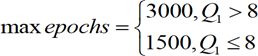
This feature extraction technique uses itself a 3-layer feedforward ANN called auto- encoder (AE). After training, the hidden layer output (y2p) for the presentation of each problem’s input pattern (y1p) is a compressed vector (Q2x 1) that can be used to replace the original input layer by a (much) smaller one, thus reducing the size of the ANN model. In this work, Q2.round.Q1/2) was adopted, being round a function that rounds the argument to the nearest integer. The implemented AE was trained using the ‘trainAutoencoder(…)’ function from MATLAB’s neural net toolbox. In order to select the best AE, 40 AEs were simulated, and their performance compared by means of the performance variable defined in sub-section 3.4. Each AE considered distinct (random) initialization parameters, half of the models used the ‘logsig’ hidden transfer functions, and the other half used the ‘satlin’ counterpart, being the identity function the common option for the output activation. In each AE, the maximum number of epochs – number of times the whole training dataset is presented to the network during learning, was defined (regardless the amount of data) by
 [2]
[2]Concerning the learning algorithm used for all AEs, no L2 weight regularization was employed, which was the only default specification not adopted in‘trainAutoencoder(…)’.
| FEATURE METHOD | F11 | F12 | F13 | F14 | F15 |
| Hidden Transfer | Parameter Initialization | Learning Algorithm | Performance Improvement | Training Mode | |
| 1 | Logistic | Midpoint (W) + Rands (b) | BP | NNC | Batch |
| 2 | Identity-Logistic | Rands | BPA | - | Mini-Batch |
| 3 | Hyperbolic Tang | Randnc (W) + Rands (b) | LM | - | Online |
| 4 | Bipolar | Randnr (W) + Rands (b) | ELM | - | - |
| 5 | Bilinear | Randsmall | mb ELM | - | - |
| 6 | Positive Sat Linear | Rand [-Δ, Δ] | I-ELM | - | - |
| 7 | Sinusoid | SVD | CI-ELM | - | - |
| 8 | Thin-Plate Spline | MB SVD | - | - | - |
| 9 | Gaussian | - | - | - | - |
| 10 | Multiquadratic | - | - | - | - |
| 11 | Radbas | - | - | - | - |
Orthogonal and Sparse Random Projections
This is another feature extraction technique aiming to reduce the dimension of input data Y1 .Q1 x .) while retaining the Euclidean distance between data points in the new feature space. This is attained by projecting all data along the (i) orthogonal or (ii) sparse random matrix . (Q1 . Q2, Q2< Q1), as described by Kasun et al. [29].
Training, Validation and Testing Datasets (feature 4)
Four distributions of data (methods) were implemented, namely pt-pv-ptt = {80-10-10, 70-15-15, 60-20-20, 50-25-25}, where pt-pv-ptt represent the amount of training, validation and testing examples as % of all learning data (.), respectively. Aiming to divide learning data into training, validation and testing subsets according to a predefined distribution pt-pv-ptt, the following algorithm was implemented (all variables are involved in these steps, including qualitative ones after converted to numeric – see 3.3.1):
· For each variable . (row) in the complete input dataset, compute its minimum and maximum values.
· Select all patterns (if some) from the learning dataset where each variable takes either its minimum or maximum value. Those patterns must be included in the training dataset, regardless what pt is. However, if the number of patterns “does not reach” pt, one should add the missing amount, providing those patterns are the ones having more variables taking extreme (minimum or maximum) values.
· In order to select the validation patterns, randomly select pv / (pv + ptt) of those patterns not belonging to the previously defined training dataset. The remainder defines the testing dataset. It might happen that the actual distribution pt– pv – ptt is not equal to the one imposed a priori (before step 1), which is due to the minimum required training patterns specified in step 2.
Input Normalization (feature 5)
The progress of training can be impaired if training data defines a region that is relatively narrow in some dimensions and elongated in others, which can be alleviated by normalizing each input variable across all data patterns. The implemented techniques are the following:
Linear Max Abs
Lachtermacher and Fuller [30] proposed a simple normalization technique given by
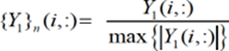 [3]
[3]where {Y1}n (., :) and Y1 (., :) are the normalized and non-normalized values of the ith input variable for all learning patterns, respectively. Notation “:” in the column index, indicate the selection of all columns (learning patterns).
Linear [0, 1] and [-1, 1]
A linear transformation for each input variable (.), mapping values in Y1(i,:) from [.*,
.*]=[min(Y1(i,:)), max(Y1(i,:))] to a generic range [a, b], is obtained from
 [4]
[4]Ranges [a, b]=[0, 1] anAd [a, b]=[-1, 1] were considered.
Nonlinear
Proposed by Pu and Mesbahi [31], although in the context of output normalization, the only nonlinear normalization method implemented for input data reads
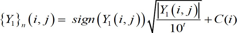 [5]
[5]where (i) Y1.i, j) is the non-normalized value of input variable . for pattern ., (ii) . is the number of digits in the integer part of Y1.i, j), (iii) sign(…) yields the sign of the argument, and (iv) .(i) is the average of two values concerning variable i, C1(i) and C2(i), where the former leads to a minimum normalized value of 0.2 for all patterns, and the latter leads to a maximum normalized value of 0.8 for all patterns.
Linear Mean Std
Tohidi and Sharifi [32] proposed the following technique
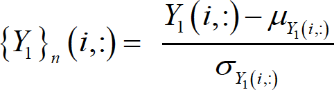 [6]
[6]where 𝜇𝑌1(𝑖,:) and 𝜎𝑌1(𝑖,:) are the mean and standard deviation of all non-normalized values (all patterns) stored by variable ..
Output Transfer Functions (feature 6)
Logistic
The most usual form of transfer functions is called Sigmoid. An example is the logistic function given by
 [7]
[7]Hyperbolic Tang
The Hyperbolic Tangent function is also of sigmoid type, being defined as
 [8]
[8]Bilinear
The implemented Bilinear function is defined as
 [9]
[9]Identity
The Identity activation is often employed in output neurons, reading
 [10]
[10]Output Normalization (feature 7)
Normalization can also be applied to the output variables so that, for instance, the amplitude of the solution surface at each variable is the same. Otherwise, training may tend to focus (at least in the earlier stages) on the solution surface with the greatest amplitude [33]. Normalization ranges not including the zero value might be a useful alternative since convergence issues may arise due to the presence of many small (close to zero) target values [34]. Four normalization methods were implemented. The first three follow eq. (4), where (i) [a, b] = 70% [.min, .max], (ii) [a, b] = 60% [.min, .max], and (iii) [a, b] = 50% [.min, .max], being [.min, .max] the output transfer function range, and [a, b] determined to be centered within [.min, .max] and to span the specified % (e.g., (b-a) =0.7 (.max – .min)). Whenever the output transfer functions are unbounded (Bilinear and Identity), it was considered [a, b] = [0, 1] and [a, b] = [-1, 1], respectively. The fourth normalization method implemented is the one described by eq. (6).
Network Architecture (feature 8)
Multi-Layer Perceptron Network (MLPN)
This is a feedforward ANN exhibiting at least one hidden layer. Fig. 2 depicts a 3-2-1 MLPN (3 input nodes, 2 hidden neurons and 1 output neuron), where units in each layer link only to some nodes located ahead. At this moment, it is appropriate to define the concept of partially- (PC) and fully-connected (FC) ANNs. In this work a FC feedforward network is characterized by having each node connected to every node in a different layer placed forward – any other type of network is said to be PC (e.g., the one in Fig. 2). According to Wilamowski [35], PC MLPNs are less powerful than MLPN where connections across layers are allowed, which usually lead to smaller networks (less neurons).
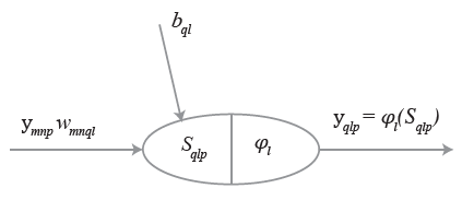
Fig. 4 represents a generic MLFN composed of . layers, where . (.= 1,…, .) is a generic layer and “ql” a generic node, being q = 1,…, Ql its position in layer . (1 is reserved to the top node). Fig. 5 represents the model of a generic neuron (. = 2,…, .), where (i) . represents the data pattern presented to the network, (ii) subscripts . = 1,…, Qn and n= 1,…, .-1 are summation indexes representing all possible nodes connecting to neuron “ql” (recall Fig. 4), (iii) bql is neuron’s bias, and (iv) wmnql represents the synaptic weight connecting units “mn” and “ql”. Neuron’s net input for the presentation of pattern . (Sqlp) is defined as
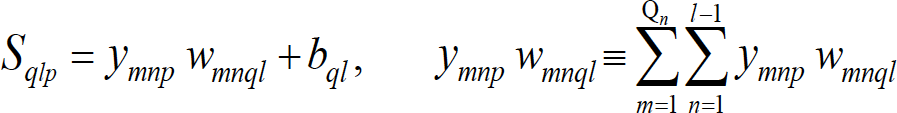 [11]
[11]where ym1p is the value of the mth network input concerning example .. The output of a generic neuron can then be written as (. = .,…, .)
 [12]
[12]where φl is the transfer function used for all neurons in layer ..
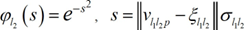
Radial-Basis Function Network (RBFN)
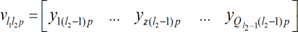
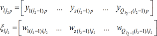
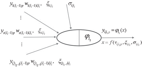
Although having similar topologies, RBFN and MLPN behave very differently due to distinct hidden neuron models – unlike the MLPN, RBFN have hidden neurons behaving differently than output neurons. According to Xie et al. [36], RBFN (i) are specially recommended in functional approximation problems when the function surface exhibits regular peaks and valleys, and (ii) perform more robustly than MLPN when dealing with noisy input data. Although traditional RBFN have 3 layers, a generic multi-hidden layer (see Fig. 4) RBFN is allowed in this work, being the generic hidden neuron’s model concerning node “l1l2” (l1 = 1,…,Ql2, l2= 2,…, .-1) presented in Fig. 6. In this model, (i) 𝑣𝑙 𝑙 𝑝 and 𝜉𝑙 𝑙 (called RBF center) are vectors of the same size (𝜉𝑧𝑙 𝑙 denotes de z component of vector 𝜉𝑙 𝑙 , and it is a network unknown), being the former associated to the presentation of data pattern ., (ii) 𝜎𝑙 𝑙 is called RBF width (a positive scalar) and also belongs, along with synaptic weights and RBF centers, to the set of network unknowns to be determined through learning, (iii) 𝜑𝑙 is the user-defined radial basis (transfer) function (RBF), described in eqs. (20)-(23), and (iv) 𝑙 𝑙 𝑝 is neuron’s output when pattern .is presented to the network. In ANNs not involving learning algorithms 1-3 in Tab. 4, vectors 𝑣𝑙 𝑙 𝑝 and 𝜉𝑙 𝑙 are defined as (two versions of 𝑣𝑙 𝑙 𝑝 where implemented and the one yielding the best results was selected)
or
 [13]
[13]and
whereas the RBFNs implemented through MATLAB neural net toolbox (involving learning algorithms 1-3 in Tab. 4) are based on the following definitions
 [14]
[14]Lastly, according to the implementation carried out for initialization purposes (described in 3.3.12), RBF center vectors per hidden layer (one per hidden neuron) are initialized as integrated in a matrix (termed RBF center matrix) having the same size of a weight matrix linking the previous layer to that specific hidden layer, and (ii) RBF widths (one per hidden neuron) are initialized as integrated in a vector (called RBF width vector) with the same size of a hypothetic bias vector.
Hidden Nodes (feature 9)
Inspired by several heuristics found in the literature for the determination of a suitable number of hidden neurons in a single hidden layer net [37-39], each value in hntest, defined in eq. (15), was tested in this work as the total number of hidden nodes in the model, i.e. the sum of nodes in all hidden layers (initially defined with the same number of neurons). The number yielding the smallest performance measure for all patterns(as defined in 3.4, with outputs and targets not postprocessed), is adopted as the best solution. The aforementioned hntest is defined by
 [15]
[15]where (i) Q1 and QL are the number of input and output nodes, respectively, (ii) . and .t are the number of learning and training patterns, respectively, and (iii) F13 is the number of features 13’s method (see Tab. 4).
Connectivity (feature 10)
For this ANN feature, three methods were implemented, namely (i) adjacent layers – only connections between adjacent layers are made possible, (ii) adjacent layers + input- output – only connections between (ii1) adjacent and (ii2) input and output layers are allowed, and (iii) fully- connected (all possible feedforward connections).
Hidden Transfer Functions (feature 11)
Besides functions (i) Logistic – eq. (7), (ii) Hyperbolic Tangent – eq. (8), and (iii) Bilinear – eq. (9), defined in 3.3.6, the ones defined next were also implemented as hidden transfer functions. During software validation it was observed that some hidden node outputs could be infinite or NaN (not-a-number in MATLAB – e.g., 0/0=Inf/Inf=NaN), due to numerical issues concerning some hidden transfer functions and/or their calculated input. In those cases, it was decided to convert infinite to unitary values and NaNs to zero (the only exception was the bipolar sigmoid function, where NaNs were converted to -1). Other implemented trick was to convert possible Gaussian function’s NaN inputs to zero.
Identity-Logistic
In Gunaratnam and Gero [40], issues associated with flat spots at the extremes of a sigmoid function were eliminated by adding a linear function to the latter, reading
 [16]
[16]Bipolar
The so-called bipolar sigmoid activation function mentioned in Lefik and Schrefler [41], ranging in [-1, 1], reads
 [17]
[17]Positive Saturating Linear
In MATLAB neural net toolbox, the so-called Positive Saturating Linear transfer function, ranging in [0, 1], is defined as
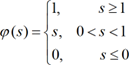 [18]
[18]Sinusoid
Concerning less popular transfer functions, reference is made in [42] to the sinusoid, which in this work was implemented as
 [19]
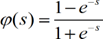
[19]Radial Basis Functions (RBF)
Although Gaussian activation often exhibits desirable properties as a RBF, several authors (e.g., [43]) have suggested several alternatives. Following nomenclature used in 3.3.8, (i) the Thin-Plate Spline function is defined by the next function is employed as Gaussian- type function when learning algorithms 4-7 are used (see Tab. 4)
 [20]
[20]the Multiquadratic function is given by
 [21]
[21]and (iv) the Gaussian-type function (called “radbas” in MATLAB toolbox) used by RBFNs trained with learning algorithms 1-3 (see Tab. 4), is defined by
 [22]
[22]where || … || denotes the Euclidean distance in all functions.
 [23]
[23]Parameter Initialization (feature 12)
The initialization of (i) weight matrices (Qa x Qb, being Qa and Qb node numbers in layers . and . being connected, respectively), (ii) bias vectors (Qb x 1), (iii) RBF center matrices (Qc-1 . Qc, being . the hidden layer that matrix refers to), and (iv) RBF width vectors (Qc x 1), are independent and in most cases randomly generated. For each ANN design carried out in
the context of each parametric analysis combo, and whenever the parameter initialization method is not the “Mini-Batch SVD”, ten distinct simulations varying (due to their random nature) initialization values are carried out, in order to find the best solution. The implemented initialization methods are described next.
Midpoint, Rands, Randnc, Randnr, Randsmall
These are all MATLAB built-in functions. Midpoint is used to initialize weight and RBF center matrices only (not vectors). All columns of the initialized matrix are equal, being each entry equal to the midpoint of the (training) output range leaving the corresponding initial layer node – recall that in weight matrices, columns represent each node in the final layer being connected, whereas rows represent each node in the initial layer counterpart. Randsgenerates random numbers with uniform distribution in [-1, 1]. Randnc (only used to initialize matrices) generates random numbers with uniform distribution in [-1, 1], and normalizes each array column to 1 (unitary Euclidean norm). Randnr (only used to initialize matrices) generates random numbers with uniform distribution in [-1, 1], and normalizes each array row to 1 (unitary Euclidean norm). Randsmall generates random numbers with uniform distribution in [-0.1, 0.1].
Rand [-lim, lim]
This function is based on the proposal in [44], and generates random numbers with uniform distribution in [-lim, lim], being lim layer-dependent and defined by
 [24]
[24]where . and . refer to the initial and final layers integrating the matrix being initialized, and . is the total number of layers in the network. In the case of a bias or RBF width vector, lim is always taken as 0.5.
SVD
Although Deng et al. [45] proposed this method for a 3-layer network, it was implemented in this work regardless the number of hidden layers.
Mini-Batch SVD
Based on [45], this scheme is an alternative version of the former SVD. Now, training data is split into min {Qb, Pt} chunks (or subsets) of equal size Pti = max {floor.Pt . Qb), 1} – floor rounds the argument to the previous integer (whenever it is decimal) or yields the argument itself, being each chunk aimed to derive Qbi = 1 hidden node.
Learning Algorithm (feature 13)
The most popular learning algorithm is called error back-propagation (BP), a first-order gradient method. Second-order gradient methods are known to have higher training speed and accuracy [46]. The most employed is called Levenberg-Marquardt (LM). All these traditional schemes were implemented using MATLAB toolbox [26].
Back-Propagation (BP, BPA), Levenberg-Marquardt (LM)
Two types of BP schemes were implemented, one with constant learning rate (BP) –‘traingd’ in MATLAB, and another with iteration-dependent rate, named BP with adaptive learning rate (BPA) – ‘traingda’ in MATLAB. The learning parameters set different than their default values are:
• Learning Rate = 0.01 / cs0.5, being cs the chunk size, as defined in 3.3.15.
• Minimum performance gradient = 0.
Concerning the LM scheme – ‘trainlm’ in MATLAB, the only learning parameter set different than its default value was the abovementioned (ii).
Extreme Learning Machine (ELM, mb ELM, I-ELM, CI-ELM)
Besides these traditional learning schemes, iterative and time-consuming by nature, four versions of a recent, powerful and non-iterative learning algorithm, called Extreme Learning Machine (ELM), were implemented (unlike initially proposed by the authors of ELM, connections across layers were allowed in this work), namely: (batch) ELM [47], Mini-Batch ELM (mb ELM) [48], Incremental ELM (I-ELM) [49], Convex Incremental ELM (CI-ELM) [50].
Performance Improvement (feature 14)
A simple and recursive approach aiming to improve ANN accuracy is called Neural Network Composite (NNC), as described in [51]. In this work, a maximum of 10 extra ANNs were added to the original one, until maximum error is not improved between successive NNC solutions. Later in this manuscript, a solution given by a single neural net might be denoted as ANN, whereas the other possible solution is called NNC.
Training Mode (feature 15)
Depending on the relative amount of training patterns, with respect to the whole training dataset, that is presented to the network in each iteration of the learning process, several types of training modes can be used, namely (i) batch or (ii) mini-batch. Whereas in the batch mode all training patterns are presented (called an epoch) to the network in each iteration, in the mini-batch counterpart the training dataset is split into several data chunks (or subsets) and in each iteration a single and new chunk is presented to the network, until (eventually) all chunks have been presented. Learning involving iterative schemes (e.g., BP- or LM-based) might require many epochs until an “optimum” design is found. The particular case of having a mini-batch mode where all chunks are composed by a single (distinct) training pattern (number of data chunks = Pt , chunk size = 1), is
called online or sequential mode. Wilson and Martinez [52] suggested that if one wants
to use mini-batch training with the same stability as online training, a rough estimate of the suitable learning rate to be used in learning algorithms such as the BP, is
, where cs is the chunk size and is the online learning rate – their proposal was adopted in this work. Based on the proposal of Liang et al. [48], the constant chunk size (cs) adopted for all chunks in mini-batch mode reads cs = min{mean.hn) + 50, Pt}, being hn a vector storing the number of hidden nodes in each hidden layer in the beginning of training and mean.hn) the average of all values in hn.
Network Performance Assessment
Several types of results were computed to assess network outputs, namely (i) maximum error, (ii) % errors greater than 3%, and (iii) performance, which are defined next. All abovementioned errors are relative errors (expressed in %) based on the following definition, concerning a single
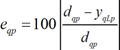 [25]
[25]where (i) dqp is the . desired (or target) output when pattern . within iteration ith (.=1,…, . ) is presented to the network, and (ii) . is net’s qth output for the same data i qLp pattern. Moreover, denominator in eq. (25) is replaced by 1 whenever |dqp| < 0.05 – dqp in the nominator keeps its real value. This exception to eq. (25) aims to reduce the apparent negative effect of large relative errors associated to target values close to zero. Even so, this trick may still lead to (relatively) large solution errors while very satisfactory results are depicted as regression plots (target vs. predicted outputs).
Maximum Error
This variable measures the maximum relative error, as defined by eq. (25), among all output variables and learning patterns.
Percentage of Errors > 3%
This variable measures the percentage of relative errors, as defined by eq. (25), among all output variables and learning patterns, that are greater than 3%.
Performance
In functional approximation problems, network performance is defined as the average relative error, as defined in eq. (25), among all output variables and data patterns being evaluated (e.g., training, all data).
Software Validation
Several benchmark datasets/functions were used to validate the developed software, involving low- to high-dimensional problems and small to large volumes of data. Due to paper length limit, validation results are not presented herein but they were made public online [53].
Parametric Analysis Results
Aiming to reduce the computing time by cutting in the number of combos to be run – note that all features combined lead to hundreds of millions of combos, the whole parametric simulation was divided into nine parametric SAs, where in each one feature 7 only takes a single value. This measure aims to make the performance ranking of all combos within each “small” analysis more “reliable”, since results used for comparison are based on target and output datasets as used in ANN training and yielded by the designed network, respectively (they are free of any postprocessing that eliminates output normalization effects on relative error values). Whereas (i) the 1st and 2nd SAs aimed to select the best methods from features 1, 2, 5, 8 and 13 (all combined), while adopting a single popular method for each of the remaining features (F3: 6, F4: 2, F6. {1 or 7}, F7: 1, F9: 1, F10: 1, F11: {3, 9 or 11}, F12: 2, F14: 1, F15: 1 – see Tabs. 2-4) – SA 1 involved learning algorithms 1-3 and SA 2 involved the ELM- based counterpart, (ii) the 3rd – 7th SAs combined all possible methods from features 3, 4, 6 and 7, and concerning all other features, adopted the methods integrating the best combination from the aforementioned first SA, (iii) the 8th SA combined all possible methods from features 11, 12 and 14, and concerning all other features, adopted the methods integrating the best combination (results compared after postprocessing) among the previous five sub- analyses, and lastly (iv) the 9th SA combined all possible methods from features 9, 10 and 15, and concerning all other features, adopted the methods integrating the best combination from the previous analysis.
ANN feature methods used in the best combo from each of the abovementioned nine parametric sub-analyses, are specified in Tab. 5 (the numbers represent the method number as in Tabs 2-4). Tab. 6 shows the corresponding relevant results for those combos, namely (i) maximum error, (ii) % errors > 3%, (iii) performance (all described in section 3, and evaluated for all learning data), (iv) total number of hidden nodes in the model, and (v) average computing time per example (including data pre- and post-processing). All results shown in Tab. 6 are based on target and output datasets computed in their original format, i.e. free of any transformations due to output normalization and/or dimensional analysis. The microprocessor used in this work has the following features: OS: Win10 Home- 64bits, RAM: 8GB, Local Disk Memory: 128GB, CPU: Intel® Core™ i5 6200U (dual-core) @ 2.30 GHz.
| SA | F1 | F2 | F3 | F4 | F5 | F6 | F7 | F8 | F9 | F10 | F11 | F12 | F13 | F14 | F15 |
| 1 | 1 | 2 | 6 | 2 | 1 | 1 | 1 | 1 | 1 | 1 | 3 | 2 | 3 | 1 | 3 |
| 2 | 1 | 2 | 6 | 2 | 3 | 7 | 1 | 2 | 1 | 1 | 9 | 2 | 7 | 1 | 3 |
| 3 | 1 | 2 | 6 | 3 | 1 | 1 | 1 | 1 | 1 | 1 | 3 | 2 | 3 | 1 | 3 |
| 4 | 1 | 2 | 6 | 2 | 1 | 1 | 2 | 1 | 1 | 1 | 3 | 2 | 3 | 1 | 3 |
| 5 | 1 | 2 | 6 | 1 | 1 | 1 | 3 | 1 | 1 | 1 | 3 | 2 | 3 | 1 | 3 |
| 6 | 1 | 2 | 6 | 2 | 1 | 7 | 4 | 1 | 1 | 1 | 3 | 2 | 3 | 1 | 3 |
| 7 | 1 | 2 | 6 | 4 | 1 | 7 | 5 | 1 | 1 | 1 | 3 | 2 | 3 | 1 | 3 |
| 8 | 1 | 2 | 6 | 4 | 1 | 7 | 5 | 1 | 1 | 1 | 3 | 2 | 3 | 1 | 3 |
| 9 | 1 | 2 | 6 | 4 | 1 | 7 | 5 | 1 | 3 | 3 | 3 | 2 | 3 | 1 | 3 |
Overall, to obtain satisfactory results, 219 ANN feature combinations were run in the parametric analysis of this problem. In 3.7, the best ANN-based model obtained is proposed to efficiently and effectively solve the real-world problem addressed. In sub-section 3.7.4, the performance results of the proposed ANN are also based on target and output datasets computed in their original format.
| SA | ANN | ||||
| Max Error (%) | Performance All Data (%) | Errors > 3% (%) | Total Hidden Nodes | Running Time / Data Point (s) | |
| 1 | 46.2 | 2.7 | 23.4 | 12 | 4.40 E -03 |
| 2 | 1598.9 | 99.2 | 90.6 | 43 | 2.58 E -04 |
| 3 | 45.5 | 2.5 | 21.9 | 12 | 1.77 E -03 |
| 4 | 141.2 | 8.7 | 34.4 | 12 | 3.23 E -04 |
| 5 | 10.1 | 1.6 | 17.2 | 12 | 1.74 E -03 |
| 6 | 253.4 | 8.9 | 31.3 | 12 | 3.04 E -03 |
| 7 | 12.4 | 1.2 | 9.4 | 12 | 7.53 E -04 |
| 8 | 108.8 | 8.4 | 31.3 | 12 | 1.44 E -03 |
| 9 | 0.2 | 0.0 | 0.0 | 12 | 1.34 E -03 |
| (a) | |||||
| SA | NNC | ||||
| Max Error (%) | Performance All Data (%) | Errors > 3% (%) | Total Hidden Nodes | Running Time / Data Point (s) | |
| 1 | 14.1 | 1.7 | 20.3 | 12 | 4.56 E -03 |
| 2 | - | - | - | - | - |
| 3 | - | - | - | - | - |
| 4 | - | - | - | - | - |
| 5 | - | - | - | - | - |
| 6 | 253.3 | 8.4 | 28.1 | 12 | 5.22 E -03 |
| 7 | 9.4 | 0.6 | 4.7 | 12 | 1.65 E -03 |
| 8 | 108.7 | 8.1 | 28.1 | 12 | 3.79 E -03 |
| 9 | - | - | - | - | - |
| (b) | |||||
Proposed ANN-Based Model
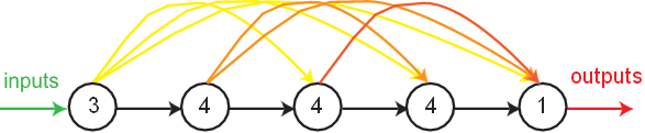
The proposed ANN is the one, among the ones simulated during the parametric analysis, exhibiting the lowest maximum error. In this case, that model was yielded by SA 9 and is characterized by the ANN feature methods {1, 2, 6, 4, 1, 7, 5, 1, 3, 3, 3, 2, 3, 1, 3} in Tabs. 2-4. Aiming to allow implementation of this model by any user, all variables/equations required for (i) data preprocessing, (ii) ANN simulation, and (iii) data postprocessing, are presented in 3.7.1-3.7.3, respectively. The proposed ANN is a MLPN with 5 layers and a distribution of nodes/layer given by 3-4-4-4-1. Concerning connectivity, the network is fully-connected (across layer connections allowed), and the hidden and output transfer functions are all HyperbolicTangent and Identity, respectively.The network was trained using the LM algorithm (1500 epochs). After design, the network computing time concerning the presentation of a single example (including data pre/postprocessing) is 1.34x10⁻³ s – Fig. 7 depicts a simplified scheme of some of network key features. Lastly, all relevant performance results concerning the proposed ANN are illustrated in3.7.4.
It is worth recalling that, in this manuscript, whenever a vector is added to a matrix, it means the former is to be added to all columns of the latter (this is valid in MATLAB).
Input Data Preprocessing
For future use of the proposed ANN to simulate new data Y1,sim (3 x Psim vector) concerning Psim
patterns, the same data preprocessing (if any) performed before training must be applied to the input dataset. That preprocessing is defined by the methods used for ANN features 2, 3 and 5 (respectively 2, 6 and 1 – see Tab. 2), which should be applied after all (eventual) qualitative variables in the input dataset are converted to numerical (using feature 1’s method). Next, the necessary preprocessing to be applied to Y1,sim, concerning features 2, 3 and 5, is fully described.
Dimensional Analysis and Dimensionality Reduction
Since neither dimensional analysis (d.a.) nor dimensionality reduction (d.r.) were carried out,
 [26]
[26]Input Normalization
After input normalization, the new input dataset  is defined as function of the previously determined
 , and they have the same size, reading
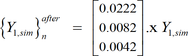 [27]
[27]where “.x” multiplies component . in the l.h.s vector by all components in row . of .1,sim.
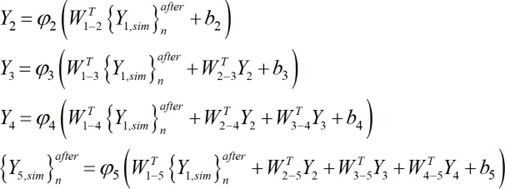
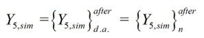
ANN-Based Analytical Model
Once determined the preprocessed input dataset {.} after (3 x .matrix), the next step1,sim nsim is to present it to the proposed ANN to obtain the predicted output dataset {Y} after5,sim n (1 x Psim vector), which will be given in the same preprocessed format of the target dataset used in learning. In order to convert the predicted outputs to their “original format” (i.e., without any transformation due to normalization or dimensional analysis – the only transformation visible will be the (eventual) qualitative variables written in their numeric representation), some postprocessing is needed, as described in detail in 3.7.3. Next, the mathematical representation of the proposed ANN is given, so that any user can implement it to determine {. } after , thus eliminating all rumors that ANNs are “black boxes”.
 [28]
[28]where
 [29]
[29]
 [30]
[30]
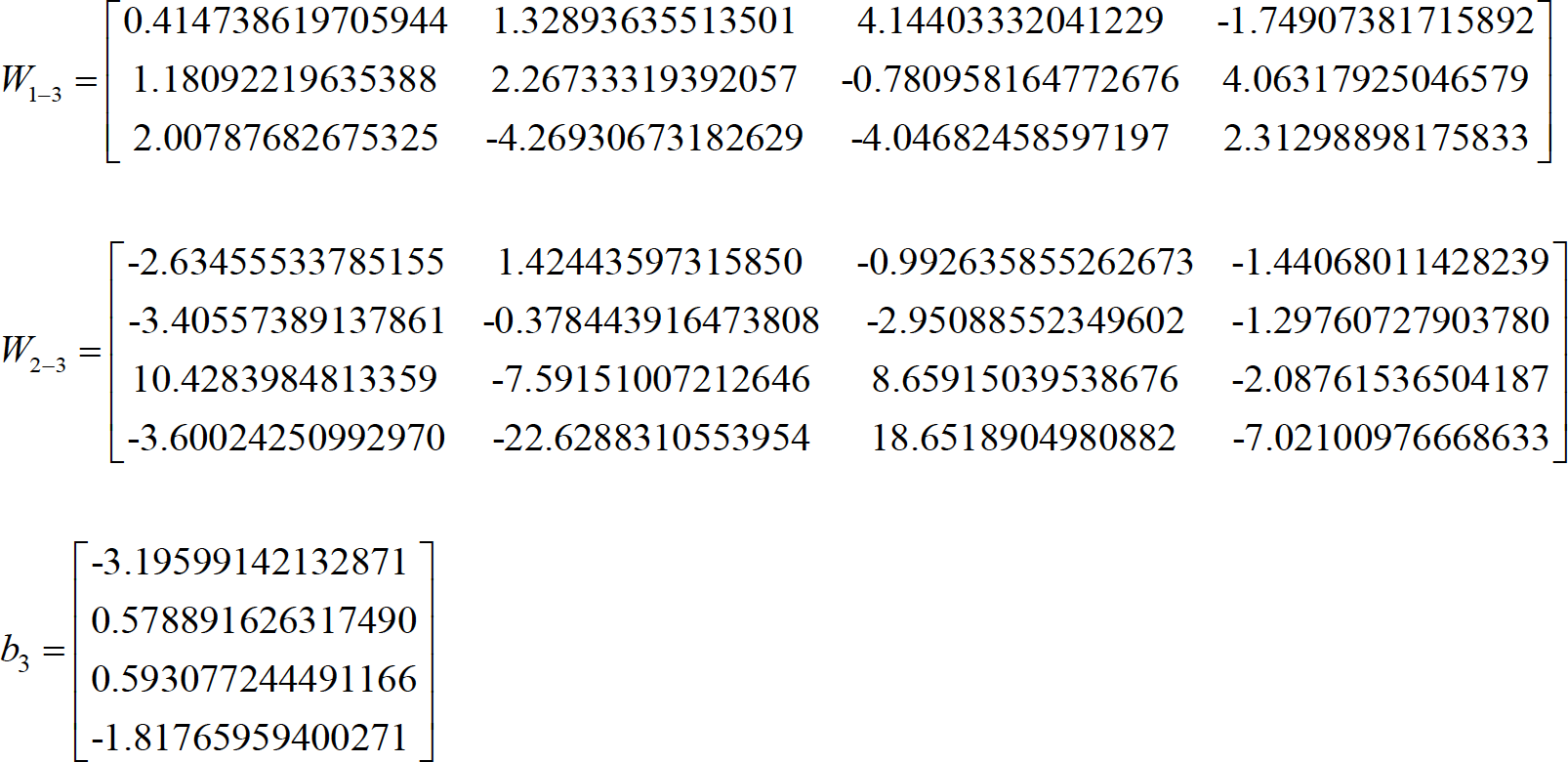 [31]
[31]
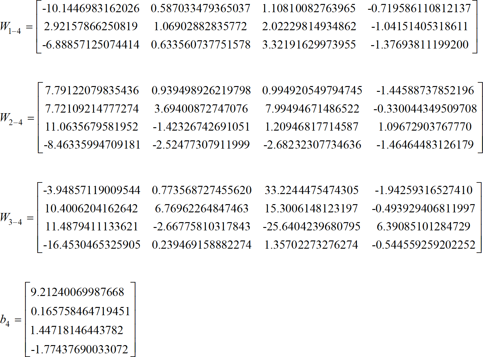 [32]
[32]
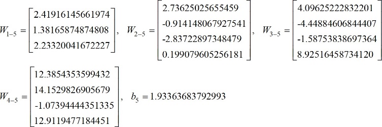 [33]
[33]Vectors and matrices presented in eqs. (30)-(33) can also be found in [54], aiming to ease their implementation by any interested reader.
Output Data Postprocessing
In order to transform the output dataset obtained by the proposed ANN, {.} after, to 5,sim n
its original format (Y5,sim), i.e. without the effects of dimensional analysis and/or output normalization (possibly) taken in target dataset preprocessing prior training, the postprocessing addressed next must be performed.
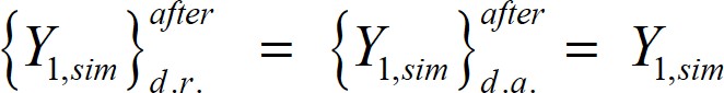
Non-normalized (just after dimensional analysis) and Original formats
Once obtained {. } after, the following relations hold for its transformation to its non- 5,sim n
normalized format {.}after(just after the dimensional analysis stage), and for latter’s5,sim da
transformation to its original format Y5,sim (with no influence of preprocessing)
 [34]
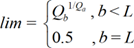
[34]since no output normalization nor dimensional analysis were carried out. Moreover, since no negative output values are physically possible for the problem addressed herein, the ANN prediction should be defined as
 [35]
[35]meaning that no structural damage exists whenever the output yielded by eq. (34) is negative.
Performance Results
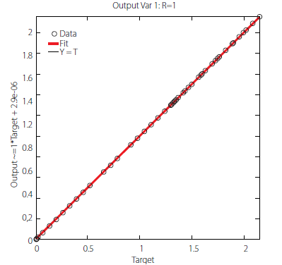
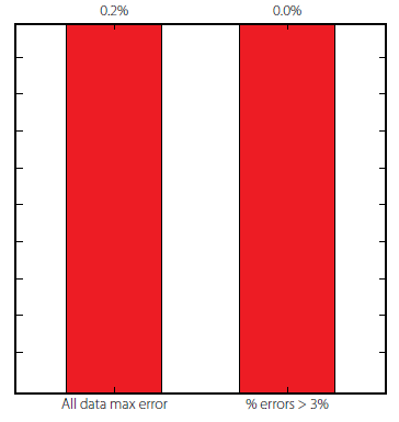
Results yielded by the proposed ANN can be found either (i) online in [18], where the target and ANN output values are provided together with the corresponding input dataset, or (ii) in terms of performance variables defined in sub-section 3.4, as presented next in the form of several graphs: (ii1) a regression plot (Fig. 8), where network target and output data are plotted, for each data point, as .- and .- coordinates, respectively – a measure of quality is given by the Pearson Correlation Coefficient (.), as defined in eq. (1); (ii2) a performance plot (Fig. 9), where performance values are displayed for several datasets; and (ii3) an error plot (Fig. 10), where values concern the maximum error and the % of errors greater than 3%, for all data. It´s worth highlighting that all graphical results just mentioned are based on target and output datasets computed in their original format, i.e. free of any transformations due to output normalization and/or dimensional analysis.
Further Testing: Prediction of Experimental Results
Aiming to test the proposed analytical model to the prediction of experimental results, three test results taken from [16] were considered, as shown in Tab. 7. Only tests I and III regard damaged members. The errors (smaller than 1%) displayed in Tab. 7 attest once again the capability of the proposed ANN-based analytical model.
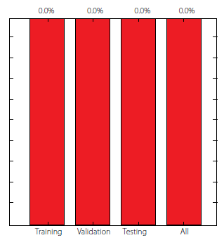
FIGURE 10. Error plot for the proposed ANN.
| TEST | Freq. 1 (Hz) | Freq. 2 (Hz) | Freq. 3 (Hz) | Real Damage Location (m) | ANN-based Damage Location (m) | Error (%) ANN vs Real |
| I | 40.142 | 117.454 | 221.441 | 1.2407 | 1.2367 | 0.3 |
| II | 42.523 | 118.771 | 231.677 | No Damage | -0.23 ⟷ 0 | 0 |
| III | 39.590 | 117.305 | 221.143 | 1.306 | 1.315 | 0.7 |
CONCLUSIONS
This paper primarily aimed to assess the potential of Artificial Neural Network (ANN) models in the prediction of damage localization in structural members, as function of their dynamic properties – the three first natural frequencies were used. Based on 64 numerical examples from damaged (mostly) and undamaged steel channel beams, an ANN-based analytical model was proposed as a highly accurate and efficient damage localization estimator. The proposed model yielded maximum errors of 0.2 and 0.7 % concerning 64 numerical and 3 experimental data points, respectively.
Since it was proved that the approach taken works well for structural members, authors’ next step (in the very near future) is to apply similar procedures to entire bridge or building structures, this time based on much larger datasets in order to provide an analytical solution with high credibility concerning its generalization capability, i.e. its capacity of giving good results for a large amount of examples (i) within the ranges considered for the input variables, and (ii) not considered during ANN development.
Acknowledgments
The 2nd and 3rd authors wish to acknowledge the support given by the Brazilian National Council for Scientific and Technological Development (CNPq) and the University of Brasília.
There are no conflicts of interest to disclose.
REFERENCES
[1] Nguyen VV, Dackermann U, Li J, Makki Alamdari M, Mustapha S, Runcie P, Ye L (2015). Damage Identification of a Concrete Arch Beam Based on Frequency Response Functions and Artificial Neural Networks. Electronic Journal of Structural Engineering, 14(1), 75-84.
[2] Onur Avci, P. O., & Abdeljaber, A. O. (2016). Self-Organizing Maps for Structural Damage Detection: A Novel Unsupervised Vibration-Based Algorithm. Journal of Performance of Constructed Facilities, 30(3), 1-11.
[3] Jin C, Jang S, Sun X, Li J, Christenson R (2016). Damage detection of a highway bridge under severe temperature changes using extended Kalman filter trained neural network. Journal of Civil Structural Health Monitoring, 6(3), 545 - 560.
[4] Chengyin L, Wu X, Wu N, Liu C (2014). Structural Damage Identification Based on Rough Sets and Artificial Neural Network, The Scientific World Journal, 2014(ID 193284), 1-9, doi: 10.1155/2014/193284
[5] MeruaneV, Mahu J (2014). Real-Time Structural Damage Assessment Using Artificial Neural Networks and Antiresonant Frequencies. Shock and Vibration, 2014 (ID 653279), 1-14, doi: 10.1155/2014/653279
[6] Structural Vibration Solutions A/S (SVS) (2018). ARTeMIS Modal 4.0®, Aalborg, Denmark.
[7] Bandara RP, Chan THT, Thambiratnam DP (2013). The Three Stage Artificial Neural Network Method for Damage Assessment of Building Structures. Australian Journal of Structural Engineering, 14 (1), 13-25.
[8] Ahmed MS (2016). Damage Detection in Reinforced Concrete Square Slabs Using Modal Analysis and Artificial Neural Network. PhD thesis, Nottingham Trent University, Nottingham, UK.
[9] Vakil-Baghmisheh M-T, Peimani M, Sadeghi MH, Ettefagh MM (2008). Crack detection in beam-like structures using genetic algorithms. Applied Soft Computing, 8(2), 1150–1160. doi:10.1016/j.asoc.2007.10.003.
[10] Aydin K, Kisi O (2015). Damage Diagnosis in Beam-Like Structures by Artificial Neural Networks. Journal of Civil Engineering and Management, 21(5), 591–604, doi:10.3846/13923730.2014.890663
[11] Kourehli SS (2015). Damage Assessment in Structures Using Incomplete Modal Data and Artificial Neural Network. International Journal of Structural Stability and Dynamics, 15(06), 1450087-1-17, doi:10.1142/s0219455414500874
[12] Nazarko P, Ziemianski L (2017). Application of artificial neural networks in the damage identification of structural elements. Computer Assisted Methods in Engineering and Science, 18(3), 175–189, Available at: http://cames.ippt.gov.pl/index.php/cames/article/view/113 (accessed on Nov 2nd 2018).
[13] Brasiliano A (2005). Identificação de Sistemas e Atualização de Modelos Numéricos com Vistas à Avaliação (in Portuguese). PhD thesis, Technology Faculty, University of Brasilia (UnB), Brasília, Brazil.
[14] Gerdau (2018). Perfil U Gerdau. [online] Available at https://www.gerdau.com/br/pt/produtos/perfil-u-gerdau#ad- image-0 [Accessed 15 Oct. 2018].
[15] ANSYS, Inc. (2018). ANSYS® – Academic Research Mechanical, Release18.1, Canonsburg, PA, USA.
[16] Marcy M, Brasiliano A, da Silva G, Doz, G (2014). Locating damages in beams with artificial neural network. Int. J. of Lifecycle Performance Engineering, 1(4), 398-413.
[17] Callister WD, Rethwisch DG (2009). Materials Science and Engineering: An Introduction (8th ed). John Wiley & Sons, Versailles, USA.
[18] Authors (2018a). data_set_ANN + results [Data set]. Zenodo, http://doi.org/10.5281/zenodo.1463849
[19] Hertzmann A, Fleet D (2012). Machine Learning and Data Mining, Lecture Notes CSC 411/D11, Computer Science Department, University of Toronto, Canada.
[20] McCulloch WS, Pitts W (1943). A logical calculus of the ideas immanent in nervous activity, Bulletin of Mathematical Biophysics, 5(4), 115–133.
[21] Hern A (2016). Google says machine learning is the future. So I tried it myself. Available at: www.theguardian.com/ technology/2016/jun/28/all (Accessed: 2 November 2016).
[22] Wilamowski BM, Irwin JD (2011). The industrial electronics handbook: IntelligentSystems, CRC Press, Boca Raton.
[23] Prieto A, Prieto B, Ortigosa EM, Ros E, Pelayo F, Ortega J, Rojas I (2016). Neural networks: An overview of early research, current frameworks and new challenges, Neurocomp., 214(Nov), 242-268.
[24] Flood I (2008). Towards the next generation of artificial neural networks for civil engineering, Advanced Engineering Informatics, 228(1), 4-14.
[25] Haykin SS (2009). Neural networks and learning machines, Prentice Hall/Pearson, NewYork.
[26] The Mathworks, Inc (2017). MATLAB R2017a, User’s Guide, Natick, USA.
[27] Bhaskar R, Nigam A (1990). Qualitative physics using dimensional analysis, Artificial Intelligence, 45(1-2), 111–73.
[28] Gholizadeh S, Pirmoz A, Attarnejad R (2011). Assessment of load carrying capacity of castellated steel beams by neural networks, Journal of Constructional Steel Research, 67(5), 770–779.
[29] Kasun LLC, Yang Y, Huang G-B, Zhang Z (2016). Dimension reduction with extreme learning machine, IEEE Transactions on Image Processing, 25(8), 3906–18.
[30] Lachtermacher G, Fuller JD (1995). Backpropagation in time-series forecasting, Journal of Forecasting 14(4), 381–393.
[31] Pu Y, Mesbahi E (2006). Application of artificial neural networks to evaluation of ultimate strength of steel panels, Engineering Structures, 28(8), 1190–1196.
[32] Tohidi S, Sharifi Y (2014). Inelastic lateral-torsional buckling capacity of corroded web opening steel beams using artificial neural networks, The IES Journal Part A: Civil & Structural Eng, 8(1), 24–40.
[33] Flood I, Kartam N (1994a). Neural Networks in Civil Engineering: I-Principals and Understanding, Journal of Computing in Civil Engineering, 8(2), 131-148.
[34] Mukherjee A, Deshpande JM, Anmala J (1996), Prediction of buckling load of columns using artificial neural networks, Journal of Structural Engineering, 122(11), 1385–7.
[35] Wilamowski BM (2009). Neural Network Architectures and Learning algorithms, IEEE Industrial Electronics Magazine, 3(4), 56-63.
[36] Xie T, Yu H, Wilamowski B (2011). Comparison between traditional neural networks and radial basis function networks, 2011 IEEE International Symposium on Industrial Electronics (ISIE), IEEE(eds), 27-30 June 2011, Gdansk University of Technology Gdansk, Poland, 1194–99.
[37] Aymerich F, Serra M (1998). Prediction of fatigue strength of composite laminates by means of neural networks. Key Eng. Materials, 144(September), 231–240.
[38] Rafiq M, Bugmann G, Easterbrook D (2001). Neural network design for engineering applications, Computers & Structures, 79(17), 1541–1552.
[39] Xu S, Chen L (2008). Novel approach for determining the optimal number of hidden layer neurons for FNN’s and its application in data mining, In: International Conference on Information Technology and Applications (ICITA), Cairns (Australia), 23–26 June 2008, pp 683–686.
[40] Gunaratnam DJ, Gero JS (1994). Effect of representation on the performance of neural networks in structural engineering applications, Computer-AidedCivilandInfrastructureEngineering,9(2),97– 108.
[41] Lefik M, Schrefler BA (2003). Artificial neural network as an incremental non-linear constitutive model for a finite element code, Computer Methods in Applied Mech and Eng, 192(28–30), 3265–3283.
[42] Bai Z, Huang G, Wang D, Wang H, Westover M (2014). Sparse extreme learning machine for classification. IEEE Transactions on Cybernetics, 44(10), 1858–70.
[43] Schwenker F, Kestler H, Palm G (2001). Three learning phases for radial-basis-function networks, Neural networks, 14(4-5), 439–58.
[44] Waszczyszyn Z (1999). Neural Networks in the Analysis and Design of Structures, CISM Courses and Lectures No. 404, Springer, Wien, New York.
[45] Deng W-Y, Bai, Z., Huang, G.-B. and Zheng, Q.-H. (2016). A fast SVD-Hidden-nodes based extreme learning machine for large-scale data Analytics, Neural Networks, 77(May), 14–28.
[46] Wilamowski BM (2011). How to not get frustrated with neural networks, 2011 IEEE International Conference on Industrial Technology (ICIT), 14-16 March, IEEE (eds),Auburn Univ., Auburn, AL.
[47] Huang G-B, Zhu Q-Y, Siew C-K (2006a). Extreme learning machine: Theory and applications, Neurocomputing, 70(1-3), 489-501.
[48] Liang N, Huang G, Saratchandran P, Sundararajan N (2006). A fast and accurate online Sequential learning algorithm for Feedforward networks, IEEE Transactions on Neural Networks, 17(6), 1411–23.
[49] Huang G, Chen L, Siew C (2006b). Universal approximation using incremental constructive feedforward networks with random hidden nodes, IEEE transactions on neural networks, 17(4), 879–92.
[50] Huang G-B, Chen L (2007). Convex incremental extreme learning machine, Neurocomputing, 70(16–18), 3056–3062.
[51] Beyer W, Liebscher M, Beer M, Graf W (2006). Neural Network Based Response Surface Methods - A Comparative Study, 5th German LS-DYNA Forum, October 2006, 29-38, Ulm.
[52] Wilson DR, Martinez TR (2003). The general inefficiency of batch training for gradient descent learning, Neural Networks, 16(10), 1429–1451.
[53] Researcher, The (2018).“Annsoftwarevalidation-report.pdf”, figshare, doi: http://doi.org/10.6084/m9.figshare.6962873
[54] Authors (2018b). W_b_arrays [Data set]. Zenodo, http://doi.org/10.5281/zenodo.1469120
Notes
Author notes
abambres@netcabo.pt